Our correspondent Peter Newnam points us to a new paper that's being talked about on the Internet, Greenhouse Effect on the Moon?, by Hertzberg et al. The gist of the paper is that no planet acts like an ideal black body, therefore any calculation that is based upon the assumption that a planet is a black body is unreliable.
We use ideal objects like black bodies, the frictionless planes, and thin lenses all the time in physics and engineering. We use these ideal objects to estimate the behavior of the real world, and as we do so, we try to keep track of the error we are likely to make as a result of our ideal assumptions. Our hope is that the error is small compared to the accuracy we require of our calculation.
When Hertzberg et al. say that planets are not ideal black bodies, they are of course correct. But in the case of the moon, we see that the black-body model they present is pretty good. The actual temperature change on the moon is 80 K to 370 K, while the black-body model they present predicts a change of 35 K to 385 K. But Hertzberg et al. point out that the average temperature of the moon is roughly 40 K higher than predicted by a black-body model, and they claim that this difference invalidates the black-body analysis of planetary temperatures.
If we want a better understanding of the moon's surface temperature, we must add the heat capacity and conductivity of the surface rocks, as well as the absorption spectrum of these rocks for short-wave and long-wave radiation. Hertzberg et al. present a graph of the moon's surface temperature versus time during the day-night cycle. We see that the surface reaches its hottest temperature after the sun has passed the zenith, which indicates that the surface rock is taking time to heat up, by virtue of its heat capacity. The surface does not have a chance to reach its equilibrium temperature in the presence of the strongest sunlight. So we are not surprised that the moon fails to reach its black-body equilibrium temperature during the day. During the night, we see the temperature is still dropping at night when the sun rises again.
The albedo of the moon for short-wave radiation is around 0.1. It absorbs 90% of incident short-wave radiation from the sun. The emissivity of the moon's surface for long-wave radiation appears to be around 0.9. It emits 90% of the radiation that a black body would radiate. If the incident radiation from the sun is a uniform 350 W/m2, we expect the moon's surface temperature to be around 280 K. But the incident heat is not uniform. The moon spends half its time very cold, at around 80 K, in which state it radiates only 0.6% of the heat it would radiate at 280 K. For less than a third of the time, the temperature is above 300 K, reaching a maximum of 370 K. At 370 K, it radiates only 300% of the heat it would radiate at 280 K. We see that the excess of heat radiated during the day cannot compensate for the deficiency of heat radiated in the cool of the night. The moon does not radiate its own heat as efficiently as it absorbs the sun's heat, and so it is warmer than a constant-temperature black-body calculation predicts.
Hertzberg et al. conclude, "The ability of common substances to store heat makes a mockery of blackbody estimates." Quite the opposite is the case. If the moon conducted and stored heat well, its surface temperature would vary less, and the black-body estimate would be more accurate.
Monday, June 7, 2010


Wednesday, June 2, 2010
Continuum Absorption Length
Our job today is to convert this graph of water vapor continuum absorption coefficient versus frequency into a graph of absorption length versus wavelength. The original graph does not give absorption coefficient directly. Instead, it gives the absorption coefficient (in inverse centimeters) divided by the density of the water vapor (in molecules per cubic centimeter) divided by the water vapor partial pressure (in atmospheres). There are twelve plots in the graph, each representing the continuum absorption at a different temperature. We zoomed in on the graph and used a cross-hair cursor to translate several of the curves into numbers. You will find our numbers in the Water Vapor page of our Climate Spreadsheet here. We plotted absorption length for three combinations of water vapor concentration (in percent of volume), vapor pressure (in millibar), and temperature (in Kelvin). We superimposed the radiation spectrum of a black body at 300 K so that we can estimate the fraction of radiated power that will be absorbed by the first few kilometers of the Earth's atmosphere.
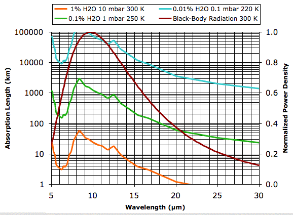
Plots of water vapor concentration versus altitude, such as this one for the Earth's atmosphere, show the concentration varying from as much as 4 % at sea-level to less than 0.0001 % at 10 km. Our plot of 1% water vapor at 10 mbar and 300 K is typical of the first 1 km of the atmosphere for 20° to 40° latitude on Earth. The absorption length of the water vapor continuum under these conditions is greater than 3 km for all wavelengths less than 16 μm. But for wavelengths greater than 20 μm the absorption length drops below 1 km. Looking at the graph, we estimate that 90% of the heat radiated straight up by the Earth's surface in these latitudes at wavelengths greater than 16 μm will be absorbed by water vapor before it reaches outer space.
Heat is radiated in all directions, which means most of it must pass through the atmosphere obliquely. Meanwhile, the atmosphere at the poles is dry, while the atmosphere in the tropics is humid. But the tropics are hotter than the poles, so that they radiate twice as much heat per square meter, and they cover a larger area too, so they contribute more to the total heat radiated by the Earth's surface.
Our guess is that almost all the heat radiated by the Earth's surface at wavelengths greater than 16 μm is absorbed by water vapor before it can reach outer space. These wavelengths represent roughly 30% of the total heat radiated by the Earth's surface.
PS. We spent several hours comparing our graphs with other calculations and measurements of water vapor absorption we found on the Internet. We believe we found good agreement between these calculations and measurements, although this agreement was not always obvious. For example, this graph from this report plots the absorption coefficient in cm2molecule−1, without mentioning the partial pressure. But we believe the graph corresponds to a partial pressure of 1 mbar. At 10.6 μm, the graph says 1.8 ×10⁻²⁵ cm2molecule−1, while Cormier et al measured 1.82 ×10⁻²² cm2molecule−1atm−1 at the same wavelength. One atmosphere is almost exactly a thousand millibar.
PPS. So far as we can tell from sites like this one, absorption of long-wave radiation by the water vapor continuum is absorption by bonds between water vapor molecules, but does not include absorption by the bonds within the water molecules. Absorption within water molecules takes place at specific frequencies, so that a plot of absorption length versus wavelength contains valleys so sharp they appear only as lines. The line at 1.1 μm, for example, is only 0.00002 μm wide (see Figure 3 here). With one such line every 0.02 μm, the lines would absorb only 0.1% of the radiation emitted by a planet surface. But such lines have a tendency to get broader when the water vapor molecules are colliding with other gas molecules, and this broadening greatly increases the fraction of long-wave radiation these lines absorb. Thus, absorption by the water vapor continuum represents some, but not all, of the absorption by water vapor.
PPPS. This history of infra-red astronomy shows that we have to get up above 3 km in a dry part of the world in order to see infra-red light from outer space. Even then, we can see only wavelengths that neither water vapor nor CO2 will absorb, and the seeing is good only when we are looking straight up. See our Vapor Versus Liquid post and its ensuing comments for more details.
Plots of water vapor concentration versus altitude, such as this one for the Earth's atmosphere, show the concentration varying from as much as 4 % at sea-level to less than 0.0001 % at 10 km. Our plot of 1% water vapor at 10 mbar and 300 K is typical of the first 1 km of the atmosphere for 20° to 40° latitude on Earth. The absorption length of the water vapor continuum under these conditions is greater than 3 km for all wavelengths less than 16 μm. But for wavelengths greater than 20 μm the absorption length drops below 1 km. Looking at the graph, we estimate that 90% of the heat radiated straight up by the Earth's surface in these latitudes at wavelengths greater than 16 μm will be absorbed by water vapor before it reaches outer space.
Heat is radiated in all directions, which means most of it must pass through the atmosphere obliquely. Meanwhile, the atmosphere at the poles is dry, while the atmosphere in the tropics is humid. But the tropics are hotter than the poles, so that they radiate twice as much heat per square meter, and they cover a larger area too, so they contribute more to the total heat radiated by the Earth's surface.
Our guess is that almost all the heat radiated by the Earth's surface at wavelengths greater than 16 μm is absorbed by water vapor before it can reach outer space. These wavelengths represent roughly 30% of the total heat radiated by the Earth's surface.
PS. We spent several hours comparing our graphs with other calculations and measurements of water vapor absorption we found on the Internet. We believe we found good agreement between these calculations and measurements, although this agreement was not always obvious. For example, this graph from this report plots the absorption coefficient in cm2molecule−1, without mentioning the partial pressure. But we believe the graph corresponds to a partial pressure of 1 mbar. At 10.6 μm, the graph says 1.8 ×10⁻²⁵ cm2molecule−1, while Cormier et al measured 1.82 ×10⁻²² cm2molecule−1atm−1 at the same wavelength. One atmosphere is almost exactly a thousand millibar.
PPS. So far as we can tell from sites like this one, absorption of long-wave radiation by the water vapor continuum is absorption by bonds between water vapor molecules, but does not include absorption by the bonds within the water molecules. Absorption within water molecules takes place at specific frequencies, so that a plot of absorption length versus wavelength contains valleys so sharp they appear only as lines. The line at 1.1 μm, for example, is only 0.00002 μm wide (see Figure 3 here). With one such line every 0.02 μm, the lines would absorb only 0.1% of the radiation emitted by a planet surface. But such lines have a tendency to get broader when the water vapor molecules are colliding with other gas molecules, and this broadening greatly increases the fraction of long-wave radiation these lines absorb. Thus, absorption by the water vapor continuum represents some, but not all, of the absorption by water vapor.
PPPS. This history of infra-red astronomy shows that we have to get up above 3 km in a dry part of the world in order to see infra-red light from outer space. Even then, we can see only wavelengths that neither water vapor nor CO2 will absorb, and the seeing is good only when we are looking straight up. See our Vapor Versus Liquid post and its ensuing comments for more details.
Thursday, May 27, 2010
Water Vapor Continuum
It may be that we can determine the absorption length of long-wave radiation in dry air with 330 ppm CO2 simply by dividing the absorption length pure CO2 by 0.00033. The absorption length of 15-μm radiation in pure CO2 is 10 mm (see CO2 Spectrum), so its absorption length in 330 ppm by volume CO2 would, according to this calculation, be 30 m.
The absorption spectrum of water vapor is not so simple. We have already presented our readers with the absorption spectrum of liquid water. But we cannot simply divide this spectrum by the fraction of water present in air and so obtain the spectrum for water vapor. Water vapor is water dissolved in air. The spectrum of liquid water applies to the Earth's oceans, and to the tiny droplets of water in clouds, but it does not apply to water vapor, as we saw in Vapor Versus Liquid. Water vapor absorbs several orders of magnitude less long-wave radiation than we would expect from dividing the liquid water spectrum by the water vapor concentration.
In liquid water, there are hydrogen bonds between each water molecule and its neighbors. These bonds absorb long-wave radiation. Hydrogen bonds are far less common in water vapor because the molecules are separated. Hydrogen bonds occur in water vapor when pairs of molecules join together to form dimers. The hydrogen bonds in these dimers absorb long-wave radiation. The chance of a water molecule finding a partner to form a dimer increases with concentration. At the same time, the number of water molecules per unit volume increases with concentration. The result is that the absorbing power of water vapor increases as the square of the concentration. Absorption by water vapor is also temperature-dependent because dimers are broken apart by kinetic energy, so colder dimers live longer and have more opportunity to absorb long-wave radiation.
There are also weak long-wave absorbing bonds between water and nitrogen, and water and oxygen. The absorption of long-wave radiation by water vapor is an on-going subject of research at many institutes. The relationship between molecules in water vapor is called the water vapor continuum. In Water vapor absorption coefficients in the 8−13-μm spectral region: a critical review (1990), Grant et al review existing measurements of the water vapor continuum spectrum. In Recent Developments in the Water Vapor Continuum (1999), Mlawer et al review existing calculations of the spectrum. The following graph of water vapor continuum absorption agrees well with measurements such as these.
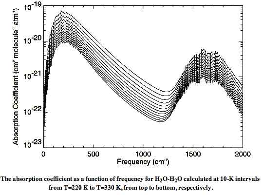
Instead of plotting the spectrum versus wavelength, this graph plots the spectrum versus the inverse of the wavelength, in units of cm−1. The spectrum itself takes the form of a quantity in units of cm2 molecule−1 atm−1, plotted for various temperatures between 220 K and 330 K. In our next post, we will convert this graph into one of absorption length versus wavelength, and show how we can calculate the absorption of long-wave radiation by water vapor in the atmosphere.
PS. Thanks to Peter Newnam for his help researching this post.
UPDATE: See CO2 Continuum for the spectrum of diluted CO2.
The absorption spectrum of water vapor is not so simple. We have already presented our readers with the absorption spectrum of liquid water. But we cannot simply divide this spectrum by the fraction of water present in air and so obtain the spectrum for water vapor. Water vapor is water dissolved in air. The spectrum of liquid water applies to the Earth's oceans, and to the tiny droplets of water in clouds, but it does not apply to water vapor, as we saw in Vapor Versus Liquid. Water vapor absorbs several orders of magnitude less long-wave radiation than we would expect from dividing the liquid water spectrum by the water vapor concentration.
In liquid water, there are hydrogen bonds between each water molecule and its neighbors. These bonds absorb long-wave radiation. Hydrogen bonds are far less common in water vapor because the molecules are separated. Hydrogen bonds occur in water vapor when pairs of molecules join together to form dimers. The hydrogen bonds in these dimers absorb long-wave radiation. The chance of a water molecule finding a partner to form a dimer increases with concentration. At the same time, the number of water molecules per unit volume increases with concentration. The result is that the absorbing power of water vapor increases as the square of the concentration. Absorption by water vapor is also temperature-dependent because dimers are broken apart by kinetic energy, so colder dimers live longer and have more opportunity to absorb long-wave radiation.
There are also weak long-wave absorbing bonds between water and nitrogen, and water and oxygen. The absorption of long-wave radiation by water vapor is an on-going subject of research at many institutes. The relationship between molecules in water vapor is called the water vapor continuum. In Water vapor absorption coefficients in the 8−13-μm spectral region: a critical review (1990), Grant et al review existing measurements of the water vapor continuum spectrum. In Recent Developments in the Water Vapor Continuum (1999), Mlawer et al review existing calculations of the spectrum. The following graph of water vapor continuum absorption agrees well with measurements such as these.
Instead of plotting the spectrum versus wavelength, this graph plots the spectrum versus the inverse of the wavelength, in units of cm−1. The spectrum itself takes the form of a quantity in units of cm2 molecule−1 atm−1, plotted for various temperatures between 220 K and 330 K. In our next post, we will convert this graph into one of absorption length versus wavelength, and show how we can calculate the absorption of long-wave radiation by water vapor in the atmosphere.
PS. Thanks to Peter Newnam for his help researching this post.
UPDATE: See CO2 Continuum for the spectrum of diluted CO2.
Wednesday, May 19, 2010
CO2 Doubling Temperature
One claim made by climatologists is that each doubling in the concentration of CO2 will cause the same increase in the Earth's surface temperature. So far as we can tell, the basis for this claim is that the absorption of radiation by greenhouse gases is "logarithmic". See Nelson, Earthguide and Wikipedia for examples. We never understood this "logarithmic" argument. We have never seen any calculations to back it up.
The greenhouse effect in our Planetary Greenhouse example is the result of logarithmic absorption by a greenhouse gas. The atmosphere contains a hypothetical gas that is opaque to some, but not all, long-wave radiation. As we showed in our previous post, successive doublings in the concentration of this gas do not cause the same increase in surface temperature. Indeed, the graph produced by our computer program shows that each successive doubling causes half as much warming as the previous doubling.
Thus logarithmic absorption alone is not sufficient justification for the existence of a "CO2 Doubling Temperature".
The greenhouse effect in our Planetary Greenhouse example is the result of logarithmic absorption by a greenhouse gas. The atmosphere contains a hypothetical gas that is opaque to some, but not all, long-wave radiation. As we showed in our previous post, successive doublings in the concentration of this gas do not cause the same increase in surface temperature. Indeed, the graph produced by our computer program shows that each successive doubling causes half as much warming as the previous doubling.
Thus logarithmic absorption alone is not sufficient justification for the existence of a "CO2 Doubling Temperature".
Monday, May 17, 2010
Planetary Greenhouse, Part Two
We continue our Planetary Greenhouse discussion. The atmosphere around our imaginary planet contains nitrogen and oxygen, which we choose because these diatomic gases are transparent to both short-wave and long-wave radiation. But the atmosphere also contains an imaginary greenhouse gas that is transparent to wavelengths shorter than λT, but absorbs longer wavelengths with constant absorption length, LT.
We wrote a computer program to determine the total heat radiated per square meter by the planet and its atmosphere. Before we can run the program, we must choose λT and LT.
Consider the absorption spectrum of pure CO2 at roughly 300 K and 100 kPa, which we present here. Between 8 μm and 11 μm the gas is transparent. The graph of radiated power versus wavelength for a black body at 300 K, which we present here, shows a peak at around 10 μm, right in the middle of CO2's transparent band. Meanwhile, the gas is at its most opaque for wavelengths greater than 13 μm. The absorption length drops to as little as 1 cm between 13μm and 17 μm, but is close to 1 m for 17 μm and higher. Let us choose λT = 13 μm and LT = 1 m.
Suppose our greenhouse gas makes up 330 ppm by volume of the atmosphere around our imaginary planet. Suppose the pressure at the planet surface is 100 kPa and the temperature is in the neighborhood of 300 K. The absorption length of the atmosphere at at the surface will be 1 m / 330 ppm = 3 km for wavelengths greater than λT. In The Upper Gas we showed how the absorption length at the surface is related to the pressure in the tropopause. With absorption length 3 km at the surface, the tropopause pressure will be 30% of the pressure at the surface, or 30 kPa. If we double the concentration of the greenhouse gas from 330 ppm to 660 ppm, the absorption length at the surface decreases to 1.5 km, and our tropopause must rise to an altitude where the pressure is only 15 kPa.
Now we can run our program, and we do so. We calculate the sum of the power radiated directly into space by the planet surface and by the troposphere. We plot this total radiated power versus the temperature of the planet surface, and we do so for a range of tropopause pressures.
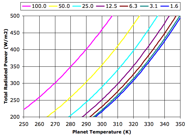
The graph legend gives tropopause pressure in kPa. Each halving of pressure corresponds to a doubling in greenhouse gas concentration. The 100 kPa graph represents the case where the concentration is so low that the troposphere is at the planet surface. The planet radiates like a black body directly into space. The 1.6 kPa graph represents a concentration so high that the the troposphere radiates hardly any heat into space. The atmosphere acts to block all radiation at wavelengths greater than λT.
For thermal equilibrium in our Planetary Greenhouse, the total power radiated into space, EP + ET, must be equal to the total power received from the sun, ES. In Solar Heat we showed how the average power reaching the Earth from the Sun was 350 W/m2, and we calculated that the surface of a black planet with no atmosphere would be 280 K. In the 100 kPa graph above, we see that the surface temperature, TP, crosses 280 K when the total radiated power is 350 W/m2.
Let us suppose that the total radiated power in our Planetary Greenhouse must be 350 W/m2. With a tropopause pressure of 50 kPa, the planet surface must be at 299 K. If we double the concentration of our greenhouse gas, the planet warms by 13 K. Subsequent doublings in concentration raise the temperature by an additional 7 K, 5 K, 3K, and 1 K.
We wrote a computer program to determine the total heat radiated per square meter by the planet and its atmosphere. Before we can run the program, we must choose λT and LT.
Consider the absorption spectrum of pure CO2 at roughly 300 K and 100 kPa, which we present here. Between 8 μm and 11 μm the gas is transparent. The graph of radiated power versus wavelength for a black body at 300 K, which we present here, shows a peak at around 10 μm, right in the middle of CO2's transparent band. Meanwhile, the gas is at its most opaque for wavelengths greater than 13 μm. The absorption length drops to as little as 1 cm between 13μm and 17 μm, but is close to 1 m for 17 μm and higher. Let us choose λT = 13 μm and LT = 1 m.
Suppose our greenhouse gas makes up 330 ppm by volume of the atmosphere around our imaginary planet. Suppose the pressure at the planet surface is 100 kPa and the temperature is in the neighborhood of 300 K. The absorption length of the atmosphere at at the surface will be 1 m / 330 ppm = 3 km for wavelengths greater than λT. In The Upper Gas we showed how the absorption length at the surface is related to the pressure in the tropopause. With absorption length 3 km at the surface, the tropopause pressure will be 30% of the pressure at the surface, or 30 kPa. If we double the concentration of the greenhouse gas from 330 ppm to 660 ppm, the absorption length at the surface decreases to 1.5 km, and our tropopause must rise to an altitude where the pressure is only 15 kPa.
Now we can run our program, and we do so. We calculate the sum of the power radiated directly into space by the planet surface and by the troposphere. We plot this total radiated power versus the temperature of the planet surface, and we do so for a range of tropopause pressures.
The graph legend gives tropopause pressure in kPa. Each halving of pressure corresponds to a doubling in greenhouse gas concentration. The 100 kPa graph represents the case where the concentration is so low that the troposphere is at the planet surface. The planet radiates like a black body directly into space. The 1.6 kPa graph represents a concentration so high that the the troposphere radiates hardly any heat into space. The atmosphere acts to block all radiation at wavelengths greater than λT.
For thermal equilibrium in our Planetary Greenhouse, the total power radiated into space, EP + ET, must be equal to the total power received from the sun, ES. In Solar Heat we showed how the average power reaching the Earth from the Sun was 350 W/m2, and we calculated that the surface of a black planet with no atmosphere would be 280 K. In the 100 kPa graph above, we see that the surface temperature, TP, crosses 280 K when the total radiated power is 350 W/m2.
Let us suppose that the total radiated power in our Planetary Greenhouse must be 350 W/m2. With a tropopause pressure of 50 kPa, the planet surface must be at 299 K. If we double the concentration of our greenhouse gas, the planet warms by 13 K. Subsequent doublings in concentration raise the temperature by an additional 7 K, 5 K, 3K, and 1 K.
Wednesday, May 12, 2010
Planetary Greenhouse
We now enhance our Extreme Greenhouse to produce a more interesting model. We incorporate the decrease in atmospheric pressure with altitude. We use our understanding of atmospheric convection to determine how atmospheric temperature changes with pressure. We enhance the properties of our greenhouse gas by making it transparent to some long-wave radiation. The result is a simple model of a Planetary Greenhouse, as shown below.
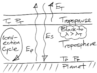
In our new model, the atmosphere continues to infinite altitude, getting thinner and thinner as we go. The lowest layer of the atmosphere is the troposphere. Above the troposphere is the tropopause. The tropopause is the layer that radiates heat into space. Above the tropopause, the atmosphere is so thin that it is transparent.
For now, we ignore day and night, and we ignore clouds. We ignore heat flowing through the solid mass of the planet. Short-wave radiation arriving from the sun passes straight through the atmosphere and is of uniform and constant power ES. The temperature and pressure at the planet surface are Tp and Pp respectively. A near-adiabatic convection cycle carries heat up through the troposphere to the tropopause, where it is radiated into space. The temperature and pressure of the tropopause are TT and PT respectively.
In our Extreme Greenhouse, the atmosphere was entirely opaque to all long-wave radiation. In our new Planetary Greenhouse, the atmosphere is transparent to all radiation with wavelength less than some threshold, λT. At greater wavelengths, a trace greenhouse gas in the atmosphere absorbs radiation. The greater the concentration of this greenhouse gas, the shorter the absorption length of the atmosphere for wavelengths greater than λT. As we saw in The Upper Gas, the shorter the absorption length, the lower the tropopause pressure. As we saw in Atmospheric Convection, the lower the tropopause pressure, the lower its temperature.
As in our Extreme Greenhouse, we assume that the planet radiates like a black body. The radiation it emits below λT passes out into space. This radiated power is EP. As we described in Black Bodies, we can use Plank's Law to determine the power radiated at all wavelengths, so we can calculate the power radiated below λT as a function of TP.
The atmospheric convection cycle allows us to calculate the temperature of the tropopause given only TP and the ratio PT/PP. The tropopause radiates power ET into space. Using Plank's Law and radiative symmetry, we can calculate the power radiated by the tropopause as a function of TT. The atmosphere emits radiation only at wavelengths greater than λT.
For thermal equilibrium, we must have the total power radiated outward by the body and the tropopause equal to the total power arriving from the sun. Thus we must have ES = EP + ET. And so we arrive at a robust model of the planetary greenhouse effect when the greenhouse gas has a step-like absorption spectrum. Given only λT and PP, we can plot a graph of EP + ET versus temperature. This graph crosses ES at the equilibrium value of TP. We wrote a computer program to calculate EP + ET versus TP for a range of tropopause pressures. You will find the program here.
In our next post, we will choose useful values for λT and ES, and we will see how doubling the concentration of our greenhouse gas affects the temperature of the planet.
In our new model, the atmosphere continues to infinite altitude, getting thinner and thinner as we go. The lowest layer of the atmosphere is the troposphere. Above the troposphere is the tropopause. The tropopause is the layer that radiates heat into space. Above the tropopause, the atmosphere is so thin that it is transparent.
For now, we ignore day and night, and we ignore clouds. We ignore heat flowing through the solid mass of the planet. Short-wave radiation arriving from the sun passes straight through the atmosphere and is of uniform and constant power ES. The temperature and pressure at the planet surface are Tp and Pp respectively. A near-adiabatic convection cycle carries heat up through the troposphere to the tropopause, where it is radiated into space. The temperature and pressure of the tropopause are TT and PT respectively.
In our Extreme Greenhouse, the atmosphere was entirely opaque to all long-wave radiation. In our new Planetary Greenhouse, the atmosphere is transparent to all radiation with wavelength less than some threshold, λT. At greater wavelengths, a trace greenhouse gas in the atmosphere absorbs radiation. The greater the concentration of this greenhouse gas, the shorter the absorption length of the atmosphere for wavelengths greater than λT. As we saw in The Upper Gas, the shorter the absorption length, the lower the tropopause pressure. As we saw in Atmospheric Convection, the lower the tropopause pressure, the lower its temperature.
As in our Extreme Greenhouse, we assume that the planet radiates like a black body. The radiation it emits below λT passes out into space. This radiated power is EP. As we described in Black Bodies, we can use Plank's Law to determine the power radiated at all wavelengths, so we can calculate the power radiated below λT as a function of TP.
The atmospheric convection cycle allows us to calculate the temperature of the tropopause given only TP and the ratio PT/PP. The tropopause radiates power ET into space. Using Plank's Law and radiative symmetry, we can calculate the power radiated by the tropopause as a function of TT. The atmosphere emits radiation only at wavelengths greater than λT.
For thermal equilibrium, we must have the total power radiated outward by the body and the tropopause equal to the total power arriving from the sun. Thus we must have ES = EP + ET. And so we arrive at a robust model of the planetary greenhouse effect when the greenhouse gas has a step-like absorption spectrum. Given only λT and PP, we can plot a graph of EP + ET versus temperature. This graph crosses ES at the equilibrium value of TP. We wrote a computer program to calculate EP + ET versus TP for a range of tropopause pressures. You will find the program here.
In our next post, we will choose useful values for λT and ES, and we will see how doubling the concentration of our greenhouse gas affects the temperature of the planet.
Wednesday, May 5, 2010
Dissipation by Convection
Now we return to our Extreme Greenhouse thought experiment. In our previous post on the subject, Work by Convection, we showed that atmospheric convection does work. We wondered where the energy for that work comes from, and where it goes to.
In our Atmospheric Convection post, the air taking part in our convection cycle warmed by 15 K while in contact with the warm surface of the Body, and cooled by 10 K while in the tropopause radiating its heat into space. The warming and cooling took place at constant pressure. The amount of heat required to warm 1 kg of a gas by 1 K at constant pressure is the heat capacity at constant pressure of the gas. Air is a close to an ideal gas. Its heat capacity at constant pressure is close to 1 kJ/kg/K at all the temperatures and pressures we are likely to encounter in the atmosphere of our Extreme Greenhouse. Each 1 kg of air absorbs 15 kJ of heat from the Body and radiates 10 kJ of heat into space. There are 5 kJ unaccounted for. These 5 kJ are converted into work.
Each kilogram of air taking part in the cycle rushes upwards with such force that it will do 5 kJ of work for us and still reach the tropopause. As it rushes upwards, it mixes with other air. Its momentum is diverted into whirlwinds. The viscosity of air is low, but it is not zero. The air moves upwards and sideways and in circles, rubbing against itself until the viscous friction it encounters consumes all the work available from convection. Viscosity turns the 5 kJ into heat.
As a result, the air in the tropopause will be warmer by 5 K than we expected with perfect, adiabatic expansion. Given that the air in the tropopause is over 100 K cooler than the air at the surface of the Body, this 5 K makes little difference to the size of our greenhouse effect. But it does mean that the air must cool in the tropopause by 15 K instead of 10 K, or else our convection cycle will not be closed. All 15 kJ of heat absorbed by the air from the Body will be radiated into space at the tropopause.
We know from our previous calculations that the atmosphere of our Extreme Greenhouse must transport 350 W/m2 from the Body surface to the tropopause (the boundary between the Filter Gas and the Upper Gas). Of these 350 W/m2, roughly 230 W/m2 will be carried directly by the heat capacity of the atmosphere, but the remaining 120 W/m2 will first be turned into work, later converted into heat by viscous action, and finally radiated into space.
The atmosphere of our Extreme Greenhouse has 120 W/m2 available to cause weather. This work is available only because the upper atmosphere is radiating heat into space. If there were no greenhouse gases in our Extreme Greenhouse, there would be no heat flow to the upper atmosphere, and no convection cycle to generate weather.
In our Atmospheric Convection post, the air taking part in our convection cycle warmed by 15 K while in contact with the warm surface of the Body, and cooled by 10 K while in the tropopause radiating its heat into space. The warming and cooling took place at constant pressure. The amount of heat required to warm 1 kg of a gas by 1 K at constant pressure is the heat capacity at constant pressure of the gas. Air is a close to an ideal gas. Its heat capacity at constant pressure is close to 1 kJ/kg/K at all the temperatures and pressures we are likely to encounter in the atmosphere of our Extreme Greenhouse. Each 1 kg of air absorbs 15 kJ of heat from the Body and radiates 10 kJ of heat into space. There are 5 kJ unaccounted for. These 5 kJ are converted into work.
Each kilogram of air taking part in the cycle rushes upwards with such force that it will do 5 kJ of work for us and still reach the tropopause. As it rushes upwards, it mixes with other air. Its momentum is diverted into whirlwinds. The viscosity of air is low, but it is not zero. The air moves upwards and sideways and in circles, rubbing against itself until the viscous friction it encounters consumes all the work available from convection. Viscosity turns the 5 kJ into heat.
As a result, the air in the tropopause will be warmer by 5 K than we expected with perfect, adiabatic expansion. Given that the air in the tropopause is over 100 K cooler than the air at the surface of the Body, this 5 K makes little difference to the size of our greenhouse effect. But it does mean that the air must cool in the tropopause by 15 K instead of 10 K, or else our convection cycle will not be closed. All 15 kJ of heat absorbed by the air from the Body will be radiated into space at the tropopause.
We know from our previous calculations that the atmosphere of our Extreme Greenhouse must transport 350 W/m2 from the Body surface to the tropopause (the boundary between the Filter Gas and the Upper Gas). Of these 350 W/m2, roughly 230 W/m2 will be carried directly by the heat capacity of the atmosphere, but the remaining 120 W/m2 will first be turned into work, later converted into heat by viscous action, and finally radiated into space.
The atmosphere of our Extreme Greenhouse has 120 W/m2 available to cause weather. This work is available only because the upper atmosphere is radiating heat into space. If there were no greenhouse gases in our Extreme Greenhouse, there would be no heat flow to the upper atmosphere, and no convection cycle to generate weather.
Subscribe to:
Posts (Atom)

