The UK parliament announced the results of its enquiry into Climategate today. Here's an excerpt.
On the much cited phrases in the leaked e-mails—"trick" and "hiding the decline"—the Committee considers that they were colloquial terms used in private e-mails and the balance of evidence is that they were not part of a systematic attempt to mislead.
Our readers are familiar with the this graph, in which the green line has been faked from 1960 onwards by deleting the tree-ring data, which went down sharply after 1960, and replacing it with thermometer data, which went up sharply after 1960. This was one version of the "trick" to "hide the decline". Another version is shown in these graphs, where the tree-ring data is simply cut short at 1960, leaving only upward graphs from that time onwards. All participants in these efforts to "hide the decline" are unashamed and open about the "trick". They say they omitted or replaced the tree-ring data because they knew it was unreliable.
I believe they are sincere. So I guess I agree with the parliament's conclusion: the scientists involved were not deliberately deceiving anyone. They believed that their graphs were consistent with the Ultimate Truth, which is that the world is getting warmer fast, and human beings are responsible for the warming. Any data that showed otherwise must, by assumption, be wrong, so it should not be plotted.
A scientist that puts his theory before the data will never discover anything new. He will never discover that he is wrong. None of us have any interest in giving him money to make discoveries because we know perfectly well he's not going to make any. The only reason to give him money is so he can keep repeating his theory to us over and over again. Putting the data first is hard. It requires mental discipline, and it is this discipline that gives science its high social standing.
Let us suppose, for the sake of argument, that a climatologist was deliberately deceiving the public about the science of global warming. This would imply that the climatologist had put the data first and reached a conclusion consistent with the data. After that, he went about telling people something opposite to the conclusion he came to. Thus we have a self-disciplined scientist who chooses to lie to people. I don't think that's possible. A self-disciplined scientist can get a job anywhere, be paid well, and sleep easily at night knowing that he has his honor intact. Why would such a person deceive anyone?
The climatologists who took part in hiding the decline are not self-disciplined in the sense I described above. They don't even know what we are talking about when we say they should put the data first. They think they are putting the data first. They don't realize what they have done wrong, other than that it got them into trouble.
All this to say: climatologists were not lying, but they have lost their reputation among other scientists, and there's no undoing that fact. As a scientist, all you have is your reputation. Once you lose it, you never get it back.
Wednesday, March 31, 2010
Tuesday, March 30, 2010
Precision by Averaging
Peter Newman points me to this claim by Chiefio that it is impossible to obtain 0.01°C precision by taking the average of measurements that are rounded to the nearest 1°C. Actually, he talks about °F, but it's the same argument. Chiefio appears to be overlooking two points. First, a thermometer that rounds to the nearest 1°C correctly must be able to distinguish between 1.49999°C and 1.50001°C. The perfectly-rounding thermometer is a perfectly-accurate thermometer. Second, every measurement has noise, and noise has some marvelous properties when it comes to taking averages.
Suppose we have an insulated box whose temperature is exactly constant at 20.23°C. We measure its temperature with a thermometer that is perfectly accurate but rounds to the nearest 1°C. So, we get a measurement of 20°C for the box, and we're wrong by 0.23°C. No matter how many perfectly-accurate thermometers we place in the box, we will always get a measurement of 20°C, and we will always be off by 0.23°C.
But thermometers are not perfect. Let's suppose we have a factory that produces thermometers that are on average perfectly accurate, but they each have an offset that is evenly-distributed in the range ±1°C. So far as we are concerned, the thermometer detects the temperature, adds the offset, and rounds to the nearest °C. To obtain the correct temperature, we subtract the offset from the thermometer reading. Half the thermometers have offset >0°C, a quarter have offset >0.5°C, and none have an offset >1°C.
Now we put 100 of these thermometers in our box and take the average of their measurements. Any thermometer with offset <0.27°C and >−0.73°C will give us a measurement of 20°C. Any thermometer with offset >0.27°C will give us a measurement of 21°C. And those with offset <−0.73°C will say 19°C. Applying our even distribution of offsets, we see that we have 13.5% saying 19°C, 50% saying 20°C, and 36.5% saying 21°C. So the average temperature of a large number of thermometers will be 0.135×19 + 0.5×20 + 0.365×21 = 20.23 °C, which is exactly correct.
In addition to permanent offsets, thermometers are subject to random errors from one measurement to the next. By taking many measurements with the same thermometer, we can obtain more precision. The underlying physical quantity tends to vary too, with short-term random fluctuations. These too we can overcome with many measurements, in many places, and at many times. The rounding error of a thermometer ends up being one of many sources of error.
In my field, we deal with rounding error all the time. We call it quantization noise. If we round to the nearest 1°C, the quantization noise is ±0.5°C, is evenly-distributed, and has standard deviation 1/√12 = 0.29 °C.
Our many evenly-distributed errors end up being added together. A consequence of the Central Limit Theorem is that the sum of many evenly-distributed errors will look like a gaussian distribution. So we tend to think of each measurement as being the correct physical value plus a random error with gaussian distribution. The arguments we have presented above will still work when applied to gaussian errors, because the gaussian distribution is symmetric.
So, despite Cheifio's skepticism, we can indeed obtain an exact measurement from a large number of thermometers that each round to the nearest °C.
Monday, March 29, 2010
Motl on CO2 Sensitivity
Lubos Motl over at The Reference Frame has an interesting post about CO2 sensitivity. He shows that there is an upper limit to how much we can expect the temperature of a body to increase when it is required to radiate an extra 1 W/m2. So far as we can tell, he implies that this radiation-based limit restricts the amount by which the Earth's surface will warm up if it is required to rid itself of an extra 1 W/m2 of heat.
But the greenhouse effect, so far as we understand it, occurs because the Earth's surface cannot radiate its heat directly into space, but instead must pass its heat to the atmosphere by convection, conduction, and radiation. The heat will be radiated when it reaches an altitude where the atmosphere becomes transparent to long-wave radiation. Black-body radiation arguments apply to the atmosphere at this transparent altitude, but not to the Earth's surface. We have not finished our analysis of the greenhouse effect, but we suspect that this transparent altitude corresponds to the tropopause, at about 12 km, where the temperature of the atmosphere stops decreasing.
In order to force heat up through 12 km of air to the tropopause, the Earth must be warmer than the tropopause. In our previous post, we showed how doubling of the concentration of a black impurity in the atmosphere might raise the altitude of transparency from 12 km to 18 km, thus increasing by 50% the distance that the Earth's heat must pass in order to reach the altitude at which it is radiated. The amount by which the Earth's surface temperature would increase under such circumstances is dominated by convection, and is only weakly dependent upon black-body radiation.
By "CO2 sensitivity", we understand climatologists to mean the amount by which the Earth's surface will warm up if we double the concentration of CO2 in the atmosphere. We don't know of any calculation of CO2 sensitivity that is consistent with our understanding of the greenhouse effect. We have looked at a half-dozen over the years, and all are similar and casual. Implementing such calculations in a computer programs and adjusting them until they fit our climate history is, to us, unconvincing. Our long series of posts on the greenhouse effect is motivated by our desire to produce a calculation for CO2 sensitivity that makes sense to us.
Tuesday, March 23, 2010
The Upper Gas
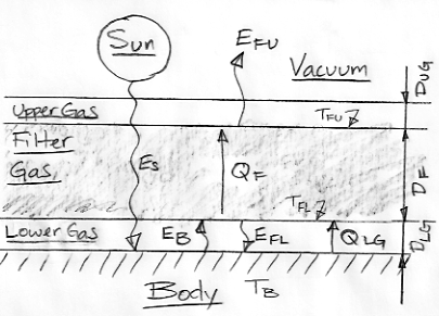
Consider the diagram we presented in Extreme Greenhouse, Part Three. The diagram shows the atmosphere divided into three layers. The Upper and Lower Gas are transparent to long-wave radiation. The Filter Gas is opaque to long-wave radiation.
Let us suppose that all the gas we portray in our diagram is air with an impurity that gives it an absorption length of 3 km for long-wave radiation when at standard temperature and pressure (STP). As we will see in later posts, this choice of 3 km will be useful when we consider CO2 in the atmosphere. Let us give our Lower Gas a thickness of 3 km. Two-thirds (1−e−1) of long-wave radiation will be absorbed in the Lower Gas. If we made the Lower Gas 30 km thick, it would be black to long-wave radiation, but we have assumed it is transparent. On the other hand, if we made the Lower Gas only 300 m thick, the lower layers of the Filter Gas would be transparent to long-wave radiation, and we have assumed them to be black. Thus our choice of 3 km for the Lower Gas is our way of approximating the 3-km absorption length of our gas.
Now consider the Upper Gas. As we present in Atmospheric Pressure, the Upper Gas is not at standard temperature and pressure. Indeed, the Upper Gas continues out to infinity as the atmosphere becomes thinner and thinner. Nevertheless, we can assign the Upper Gas a thickness in terms of the mass of air it contains. A 3-km high column of air 1 m2 in cross-section, and at STP, weighs 3000 kg and absorbs two-thirds of long-wave radiation. To the first approximation, this same mass of air will absorb two-thirds of long-wave radiation regardless of its pressure and temperature. So let us say that the Upper Gas contains 3000 kg of air per square meter. As we showed in our previous post, 3,000 kg of air above every square meter means a 30 kN weight for every square meter, so the pressure at the base of the Upper Gas is 30 kPa. The Upper Gas allows one-third of long-wave radiation from the Filter Gas to pass out into space.
The Upper Gas continues to infinity, but its base is at an altitude where the pressure is 30 Pa. According to our previous calculations, this altitude will be roughly 12 km. Given that our Lower Gas extends to 3 km and our Upper Gas begins at 12 km, this leaves our Filter Gas with a thickness of 9 km.
Now suppose we double the concentration of the long-wave absorbing impurity in our gas. The absorption length of the gas will halve. The Lower Gas will be 1.5 km thick. The Upper Gas will begin at 15 Pa pressure, or 19 km altitude. Our Filter Gas will now be 17.5 km thick. Decreasing the absorption length of our gas causes the Filter Layer to grow. As we determined previously, a thicker Filter Layer means a warmer Body.
From now on, we will refer to the boundary between the Upper Gas and the Filter Gas as the tropopause of our atmosphere. At this altitude, our atmosphere stops getting colder as we ascend. The Earth's atmosphere has a tropopause as well, and we will see in subsequent posts that it is the altitude of the tropopause that dictates the strength of the greenhouse effect.
Tuesday, March 16, 2010
Atmospheric Weight
At sea-level, the Earth's atmosphere exerts a 100 kN force upon every square meter of the ground. That's a ten-tonne weight per square meter. How does this ten-tonne weight relate to the weight of the air column above that one square meter? In our previous post we concluded that pressure, p, varied with altitude, y according to,
p = 105 e−y/104
Furthermore, we concluded that the density of the atmosphere, ρ, was related to pressure according to,
ρ = p/f, with f = 105 Nm/kg
When we combine these two equations, we arrive at,
ρ = e−y/104
Consider our infinitesimal atmospheric element, which you can see here. Its infinitesimal mass, dm, is given by,
dm = Aρdy = Ae−y/104dy
Let's imagine going from sea-level to infinity, adding together the masses of all the infinitesimal elements as we go. That is to say: let us integrate dm with respect to y for y = 0 to ∞, and let's also assume A = 1 m2, so we obtain the mass of air above one square meter.
0∫∞ Ae−y/104dy = 104 kg
So, there we have it: the mass of air above one square meter at sea-level is 10,000 kg, or ten tonnes. The pressure of the atmosphere at sea-level is equal to the weight of the atmosphere above each square meter. Indeed, the same is true at any altitude: the pressure at any altitude is equal to the weight per square meter of the atmosphere above that altitude. This conclusion is important for our future efforts to determine the absorbing power of the atmosphere. If we have radiation at altitude y, we know what mass of air this radiation must pass through to get to outer space.
Suppose the atmosphere were incompressible, like water, but we had just as much of it as we do now. This atmosphere's total mass is the same, but its density would be 1 kg/m3 all the way through. It's height would be 10 km. As it is, we have 68% of the atmosphere contained in the first 10 km and 99% contained in the first 46 km.
In a future post, we'll see if we can determine the altitude at which the upper atmosphere becomes so thin that it is transparent to its own long-wave radiation.
Tuesday, March 9, 2010
Atmospheric Pressure
Our extreme greenhouse argument has reached the point where we need a relationship between atmospheric pressure and altitude. Those of you who are not scientists might enjoy this simple demonstration of the power of infinitesimal calculus. The drawing below shows an element of the atmosphere at altitude y. The element has horizontal cross-sectional area A and a vertical thickness dy. The gas within the element has density ρ. The mass of the element is therefore ρAdy If we let g represent the acceleration due to gravity, the weight of our element is ρAgdy.
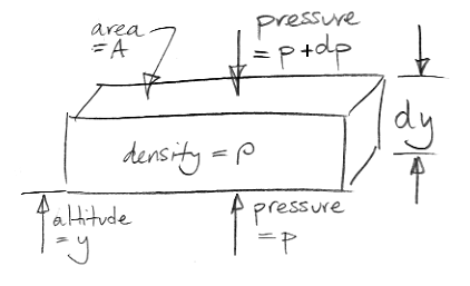
What holds up the weight of our element? The only external forces acting upon our element are pressure below and pressure above. We stop any argument about sheer forces at the edges by saying that all edge effects are negligible because dy is infinitely small. (That's our first use of the infinitesimal part of calculus.)
We assume our element is at rest with respect to the Earth. The pressure pushing up from below must be slightly greater than the pressure pushing down from above in order to hold up the weight of the element. Our drawing gives the pressure above as p+dp, where dp is a small difference in pressure. We will find that dp is negative. The upward pressure force is Ap. The downward pressure force is A(p+dp). For the vertical forces upon our element to balance we have,
Ap = A(p+dp) + ρAgdy
⇒ dp = −ρgdy
⇒ dp/dy = −ρg
The term on the bottom left is the "derivative of p with respect to y", or the "rate of change of pressure with altitude." We see that the derivative is independent of A, and is always negative.
We now introduce a further complication: the density of a gas depends upon pressure and temperature. According to Boyle's Law, p/ρT is constant, where T is absolute temperature. If we halve the pressure and keep the temperature constant, the density must also halve. We know that pressure drops to zero as we go up through the Earth's atmosphere. We also know that temperature drops from around 290 K at the surface to 210 K at the top of the troposphere. After that, the temperature rises again. If we assume temperature is constant at 250 K, we'll be right to ± 20%, which is good enough for our purposes, and simplifies our mathematics significantly.
Thus we assume there is a constant f such that f = p/ρ as we go up through the atmosphere. The density of air at atmospheric pressure and 250 K is roughly 1 kg/m3. Atmospheric pressure is 100 kPa (roughly ten tonnes per square meter). Thus f = 100 kPa / 1 kgm−3 = 105 Nm/kg, and for other pressures we have ρ = p/f. Our differential equation becomes,
dp/dy = −pg/f
The only relationship between p and y that satisfies our differential equation is the following, where we have p proportional to the natural number, e = 2.72, raised to a negative power in y.
p = p0e−gy/f
where p0 is the pressure when y = 0, which is 100 kPa. Gravity at the surface of the Earth is roughly 10 m/s2. The radius of the Earth is around 6,000 km, and gravity is proportional to the inverse square of distance, so gravity at the top of a 100-km thick atmosphere would be only 3% less. We can assume gravity is constant. Now we have,
p = 105 e−y/10 km Pa
Every 10-km increase in altitude causes the pressure to drop by 63%. At altitude 10 km, p = 37 kPa. At 20 km, p = 14 kPa. At 100 km, p = 0.005 kPa.
We will discuss our solution further in a later post. Until then, I invite you to consider the following questions. How is the weight of the atmosphere related to the pressure at sea-level? What altitude includes 99% of all atmospheric gas? If air was an incompressible fluid, so that ρ = 1 kg/m3 for all T and p, how deep would the atmosphere be?
UPDATE: For 1 kg of air we have p/ρT = R, where R is the specific gas constant for air and is equal to 287 J/kgK. Thus f = RT, and our equation for pressure with altitude becomes p = p0e−gy/RT. The altitude at which the pressure drops by 63% is a function only of temperature, a fact that emerges in the comments of Adiabatic Balloons.
UPDATE: Because most of the mass of the atmosphere is below 10 km, we should bias our average temperature more towards the surface temperature. Let us use 260 K for the average air temperature on a warm day. Using 287 J/kgK for R, we estimate the pressure will drop by 63% in 6.5 km instead of 10 km, which is consistent with typical conditions in our atmosphere.
Thursday, March 4, 2010
Truth by Law
Peter Newnam points us to Memorandum submitted by Dr Sonja Boehmer-Christiansen (CRU 26).
"This cause of environmental protection had from the start natural allies in the EU Commission, United Nation and World Bank. CRU, working for the UK government and hence the IPCC, was expected to support the hypothesis of man-made, dangerous warming caused by carbon dioxide, a hypothesis it had helped to formulate in the late 1980s and which became "true" in international law with the adoption of the 1992 Framework Convention on Climate Change."
That's an interesting concept: the truth of anthropogenic global warming was enshrined in international law. In the United States, the EPA has decided that carbon dioxide is dangerous to human health. Once these statements about the natural world become enshrined in the law, any opposition to the statements becomes opposition to the law. Opposition to a law is not, in itself, a crime. But the opposer now finds himself being compared to someone who is making excuses for not obeying the law. Oil companies were placed in that position by the international laws, and automobile companies are in that position with respect to our EPA.
I'm not complaining: the truth is coming out in the end.
Subscribe to:
Posts (Atom)
