Carbon Cycle: With Ten Petagrams per Year

Today we use our model of the Earth's carbon cycle to show us what will happen if we start adding ten petagrams of carbon to the atmosphere each year by burning fossil fuels. Ten petagrams is roughly the amount we emitted in 2015, so we are going to see how this addition would affect the concentration of CO2 in the atmosphere if it began suddenly, continued for thousands of years, and was the only phenomenon affecting change in the carbon cycle. In particular, our calculation assumes that the temperature of the atmosphere and the ocean remain constant, which may not be true if rising CO2 concentration enhances the greenhouse effect.

We begin with the carbon cycle in its natural, equilibrium state. The concentration of CO2 in the atmosphere is 300 ppm, which means it contains 650 Pg of carbon. The oceanic carbon reservoir, meanwhile, contains 77,000 Pg. Each year, the ocean emits 37 Pg into the atmosphere, and absorbs 37 Pg from the atmosphere. But now we start adding an extra 10 Pg/yr to the atmosphere by burning fossil fuels. In the the numerical equations that describe our carbon cycle, we set m_F = 10 Pg/yr. You can download our carbon cycle spreadsheet here. In it, you will find the following plot, along with our calculations.


Figure: Atmospheric and Oceanic Carbon Mass versus Time, with Ten Petagrams per Year Fossil Fuel Emissions. The time scale is logarithmic. Note that 1 Eg = 1,000 Pg. Click to enlarge.
During the first ten years, the total mass of carbon entering the atmosphere each year is 47 Pg/yr. But the mass absorbed by the oceans remains 37 Pg/yr. The mass of carbon in the atmosphere increases by 10 Pg/yr.

After ten years, we have emitted 100 Pg by burning fossil fuels. The mass of carbon in the atmosphere has increased by 80 Pg to 730 Pg. The rate at which carbon is absorbed by the ocean has increased in proportion, because there are more CO2 molecules available to absorb. The ocean now absorbs 41 Pg/yr. With 37 Pg/yr emitted by the ocean, and 10 Pg/yr emitted by burning fossil fuels, the carbon mass of the atmosphere increases by 6 Pg/yr.

After a hundred years, we have emitted 1,000 Pg by burning fossil fuels. The mass of carbon in the atmosphere has increased by 180 Pg to 830 Pg. The rate at which atmospheric carbon enters the oceanic reservoir is 47 Pg/yr. The mass of the oceanic reservoir itself has increased by 820 kg to 77,820 kg, which is only 1%. The rate at which oceanic carbon emerges into the atmosphere is still close to 37 Pg/yr. The atmosphere is in equilibrium: carbon enters at 47 Pg/yr and leaves at 47 Pg/yr. Its carbon mass increases only by 0.1 Pg/yr.

After one thousand years, the mass of carbon in the oceanic reservoir has increased by 13% to 87,000 Pg. The rate at which the ocean emits carbon into the atmosphere has increased by 13% to 42 Pg/yr. The mass of carbon in the atmosphere has risen to 910 Pg, and every year 52 Pg of atmospheric carbon is absorbed by the oceanic reservoir. The atmosphere is still in equilibrium with the ocean: each year 52 Pg enters and 52 Pg leaves. Its carbon mass continues to increase by only 0.1 Pg/yr, while the carbon in the oceanic reservoir increases by 10 Pg/yr.

After six thousand years, the mass of carbon in the atmosphere has doubled, and the mass in the oceanic reservoir has almost doubled. The plot below shows how atmospheric CO2 concentration increases with time for the same scenario.


Figure: Atmospheric CO2 Concentration in Response to Emission of 10 Pg/yr of Carbon by Burning Fossil Fuels. Units are parts per million by volume. Click to enlarge.
Burning fossil fuels at the rate we are going today, it would take 100 years to raise the concentration of CO2 in our natural, equilibrium atmosphere from 300 ppmv to 400 ppmv, and 6,000 years to raise it from 300 ppmv to 600 ppmv.

Carbon Cycle: Equations and Diagram

Suppose human beings start to add carbon to our natural, equilibrium atmosphere at a rate m_F by burning fossil fuels. We will express m_F in petagrams of carbon per year, or Pg/yr. Note that we have been working with carbon masses, not CO2 masses, but we can convert atmospheric carbon mass to atmospheric CO2 mass simply by multiplying by 3.7, which is the ratio of the molar mass of CO2 to the atomic mass of carbon-12. With the addition of m_F, our carbon cycle now looks like the diagram below. The time t = 0 yr is the moment just before we start we start adding m_F to the atmosphere.


Or, expressed as two differential equations, it looks like this:


We can solve these differential equations in the same way we already solved those of carbon-14 concentration. Examining the equations, we see that we can obtain the behavior of non-radioactive carbon by setting the decay constant, γ, to zero and inserting the the human emission of carbon in place of the cosmic ray creation of carbon-14. More convenient than the analytic solution for our purposes, however, is a numerical solution that we can implement in a spreadsheet and combine with the historical and projected values for m_F as our study progresses.

In the numerical solution, we pick a time step small enough that changes in the masses and transfer rates are negligible during the step. Suppose our step is δt. Provided δt is small enough, we can assume, for example, that m_A during each step is equal to k_A times the value of M_A at the beginning of the step. We do not have to account for the fact that M_A may be changing during the step, because the time step is so small these changes will be negligible compared to M_A. For our carbon cycle, it turns out that one year is always a small enough time step, and in long, slow developments, ten years is small enough.

The following equations are the numerical equivalents of our differential equations. They show how we calculate M_A and M_R at time t+δt using their values at time t.


The current rate at which humans emit carbon by burning fossil fuels is close to, 10 Pg/yr. In our next post, we will set m_F to a constant 10 Pg/yr and calculate how our natural, equilibrium atmosphere responds over ten thousand years.

PS. If you find our carbon cycle drawing too confusing and drab, you can try this one drawn by my youngest son.

Carbon Cycle: Rate of Transfer

Our study of the radioactive isotope carbon-14, which we began in Carbon-14: Origins and Reservoir, led us to the conclusion that roughly one in every eighteen atmospheric carbon atoms are absorbed by a vast oceanic reservoir each year. When the atmosphere and the reservoir are in equilibrium, the same amount of carbon flows out of the reservoir as into it, so that the mass of carbon in the atmosphere remains constant. But the oceanic reservoir contains over one hundred times as much carbon as the atmosphere.

We now embark upon a series of posts in which we calculate the effect of mankind's carbon emissions upon the atmospheric CO2 concentration. Our starting point for these calculations will be the natural, equilibrium atmosphere and oceans of the late nineteenth century. This atmosphere contains 300 ppmv CO2, which implies a total atmospheric carbon mass of 650 Pg (see here). The oceanic reservoir contains 77,000 Pg, and each year 37 Pg of carbon is exchanged between the atmosphere and the reservoir (see here).

As we showed in our previous post, the probability of an atmospheric carbon atom being transferred into the oceanic reservoir is independent of the number of carbon atoms in the atmosphere. The number of carbon atoms moving into the reservoir is equal to the total number of carbon atoms in the atmosphere divided by eighteen. If we have twice as many carbon atoms, the rate at which they move into the oceanic reservoir will double. If m_A is the mass of carbon moving into the reservoir every year, and M_A is the mass of carbon in the atmosphere, we must have:

m_A = k_AM_A, where k_A = 37 Pg/yr ÷ 650 Pg = 0.057 Pg/yr/Pg.

The probability of a carbon atom in the oceanic reservoir being released into the atmosphere is likewise independent of the number of carbon atoms in the reservoir. If m_R is the mass of carbon leaving the reservoir every year and M_R is the mass of carbon in the reservoir, we must have:

m_R = k_RM_R, where k_R = 37 Pg/yr ÷ 77,000 Pg = 0.00048 Pg/yr/Pg.

If we were to double suddenly the mass of carbon in the atmosphere, carbon would start to move into the oceanic reservoir at double the rate. The graph of atmospheric carbon dioxide concentration would look almost exactly like the graph of carbon-14 concentration after the nuclear bomb tests, which we present here. The movement of carbon between the atmosphere and the oceanic reservoir is governed by almost exactly the same equations as the movement of carbon-14. The only difference is that carbon-14 decays, while carbon-12 lasts forever.

UPDATE: The above calculations are consistent with Henry's Law of gasses dissolving in liquids. Henry's Law applies when the concentration of gas in the liquid has reached equilibrium at a particular temperature with the concentration of gas above the liquid. At equilibrium, the rate at which the liquid emits the gas is equal to the rate at which the liquid absorbs the gas. Henry's Law states that the equilibrium concentration of the gas in the liquid at a particular temperature is proportional to the partial pressure of the gas above the liquid. According to Boyle's Law, the partial pressure of a gas at a particular temperature is proportional to the number of gas molecules per unit volume. In our rate of transfer equations, the rate at which CO2 is absorbed by the ocean is proportional to the concentration of CO2 in the atmosphere, and the rate at which CO2 is emitted is proportional to the concentration in the liquid. If we double the concentration of CO2 in the atmosphere, our equations tell us that the rate of emission by the oceans will equal the rate of absorption only if the concentration of CO2 in the oceans also doubles, which is precisely what Henry's Law requires. Of course, we have not yet considered how changing the temperature of the atmosphere and ocean will affect the rates of transfer, but we will get to that later.

Carbon-14: Probability of Exchange

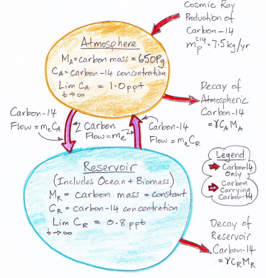
In the carbon cycle of our natural, equilibrium atmosphere, each carbon atom in the atmosphere has a certain probability each year of being absorbed by the reservoir. We call this the probability of exchange in the atmosphere. According to our calculations, 37 Pg of carbon is absorbed by the reservoir each year. Meanwhile, the total mass of carbon in the atmosphere is 650 Pg. To the first approximation, the probability of exchange in the atmosphere is 5.7% per year.

Likewise, a carbon atom in the reservoir has a probability of being released into the atmosphere each year. We have 37 Pg of carbon emerging from the reservoir each year, and the reservoir contains 77,000 Pg of carbon, so the probability of exchange for the reservoir is 0.048% per year.

Almost all carbon in the atmosphere is bound up in CO2. In our previous post we showed that the reservoir is the deep ocean. When a carbon atom enters the deep ocean, it does so as part of a CO2 molecule. The CO2 molecule arrives by chance at the ocean surface, and by further chance it dissolves into the salty water. The CO2 molecule turns into some kind of carbonate ion. This ion mixes down through the top thousand meters of water until it reaches the deep ocean. The carbon atom is now part of the reservoir. The probability of this happening each year is 5.7% for each and every CO2 molecule in the atmosphere.

Likewise, the probability of any carbon atom in the reservoir emerging into the atmosphere as part of a new CO2 molecule each year is 0.048%. The molecule or ion containing the carbon atom mixes up through the top one thousand meters of the ocean, arrives by chance at the surface, and by further chance emerges from the surface as an atmospheric CO2 molecule. (See UPDATE below for discussion of ocean chemistry.)

The exchange of carbon between the atmosphere and the ocean is a first-order chemical process. During the process, each carbon atom is acting alone. It does not require the cooperation of any catalyst to permit it to be dissolved in saltwater or released from saltwater. If we were to double the number of CO2 molecules in the atmosphere, so that six hundred out of every million air molecules were CO2 instead of only three hundred, the probability of any one of them being absorbed by the reservoir each year would remain the same.

If the reservoir were something more complex than the ocean, such as a forest, we would be unable to assert that the probability of exchange was unaffected by the number of CO2 molecules in the atmosphere. A forest needs water and sunlight to convert CO2 into sugar and oxygen. If we double the number of CO2 molecules in the atmosphere, we might find that CO2 molecules are lining up inside forest leaves waiting for enough water and sunlight to arrive before they are turned into plant matter. But our reservoir is the ocean, and entering and leaving it is a statistical process in which each carbon atom acts in isolation.

So far, we have assumed that the atmosphere and reservoir are staying at the same temperature. They could be at different temperatures, but they are neither warming nor cooling. But we note that the probability of exchange is strongly affected by temperature. We have only to look at the decreasing solubility of CO2 in water with temperature, as presented here, to see that this strong effect must exist.

For now, we assume our natural, equilibrium atmosphere, and its carbon reservoir, are neither cooling nor warming. The probability of exchange in the atmosphere remains constant at 5.7% per year, even if we halve or double the atmosphere's CO2 concentration. The probability of exchange in the reservoir remains constant at 0.048% per year, even if the mass of carbon in the reservoir halves or doubles. The probability of exchange is independent of concentration.

This concludes our series of posts on carbon-14. In our upcoming posts, we will apply what carbon-14 has taught us about the Earth's carbon cycle to predict how human CO2 emissions will affect the CO2 concentration of the atmosphere.

UPDATE [08-NOV-16]: In many gas-liquid systems, changes in concentration or acidity can change the probability of emission for a dissolved gas molecule. This variation in probability is possible when the dissolved gas appears as several species in the liquid, some of which cannot emit a gas molecule, while others can. When the relative concentrations of these species changes, the probability of a dissolved gas molecule being emitted also changes. For example, if a gas dissolves into two species A and B in equal proportion, and A has a 10% per year probability of emission while B has a 0% probability, the average probability is 5% per year. If we add acid to the system and the ratio of the two becomes 75% A and 25% B, the probability of emission for each species remains the same, but the average probability rises to 7.5% per year. Our carbon-cycle model is based upon the assumption that the atmosphere-ocean system does not exhibit concentration-dependent nor acidity-dependent probability of emission. Let us justify our assumption with a brief discussion of ocean chemistry.

The top layer of the ocean is saturated with calcium carbonate (CaCO3). The CaCO3 co-exists with the carbonate ions created by CO2 dissolved in water. In Figure 5.6 of Carbonate Equilibria we see the pH of a liquid saturated with calcium carbonate is around 8.5 (log of the H⁺ concentration is −8.5) for CO2 partial pressure of 300 ppmv (log of CO2 partial pressure is −3.5). The pH of our contemporary ocean is around 8.2, while the pH of a system of only CO2 and water is around 5.8. Continuing with Figure 5.6, for CO2 partial pressures in the range 100 ppmv to 10,000 ppmv (log of CO2 partial pressure is −4 to −2) the carbon content of the solution is dominated by HCO3⁻. The concentration of HCO3⁻ increases in proportion to the partial pressure of CO2 (its slope is 1.0 in the log-log plot). The concentration of HCO3⁻ is 2.0 times that of Ca²⁺ throughout the range 100 ppmv to 10,000 ppmv (see Table 5.1 Case 2 for numerical values). As we increase the partial pressure of CO2, an equal number of of CaCO3 and CO2 molecules dissolve. Each CaCO3 molecule that dissolves adds one Ca²⁺ ion, one HCO3⁻ ion, and one OH⁻ ion to the solution. Each CO2 molecule that dissolves contributes one HCO3⁻ ion and one H⁺ ion. The OH⁻ and H⁺ ions combine to form H2O, leaving the other ions in solution. The HCO3⁻ concentration, the dissolved CO2 concentration, and the dissolved CaCO3 concentration all increase in proportion to the partial pressure of CO2. As seawater changes temperature and pressure, the saturation concentration of CaCO3 changes, and CaCO3 can precipitate, as it does in the Persian Gulf, staining the water white.

When a gas and liquid are at equilibrium, there is as much gas entering the liquid per unit time as there is leaving it. Because gaseous CO2 has only one species, its probability of absorption into the ocean does not vary with its concentration. When we double the concentration of atmospheric CO2 from 300 ppmv to 600 ppmv, we double the rate at which it enters the ocean. When the ocean attains a new equilibrium with the 600-ppmv CO2 atmosphere, the rate at which CO2 is emitted by the ocean must be double the rate for 300 ppmv. At the same time, using the CaCO3-CO2-water system as our guide, we see that the concentration of dissolved CO2 will double for this doubling of atmospheric concentration. The doubling of dissolved concentration combined with the doubling of emission tells us that the probability of emission for CO2 molecules in the ocean is constant from 300 ppmv to 600 ppmv.

Another way to model the atmosphere-ocean system is to ignore the calcium carbonate and instead use a CO2-water system with added OH⁻, such as might come from mixing NaOH with the water. We add OH⁻ in order to increase the pH of the system from 5.8, which applies to the CO2-water system alone, to 8.2, which applies to the ocean. This OH-CO2-water system exhibits more complex behavior in the range 100 ppmv to 1000 ppmv than the CaCO3-CO2-water system. The dissolved CO2 concentration does not increase in proportion to the atmospheric concentration. So far as we can tell, this OH-CO2-water model is what climate scientists are using when they conclude that the ocean will not absorb our CO2 emissions in proportion to atmospheric CO2 concentration. They express its non-linear behavior with a number they call the Revelle Factor. We do not understand why they prefer an OH-CO2-water model to the CaCO3-CO2-water model, nor have we seen in the climate science literature any plots like those of Figure 5.4 or Figure 5.6 for an OH-CO2-water system. The closest we have seen any promoter of the Revelle Factor come to plotting such graphs is here, but that author had no explanation for why they used the OH-CO2-water system instead of the CaCO3-CO2-water system.

Carbon-14: The Reservoir Is the Ocean

Up to now, we have guessed that the carbon-14 reservoir in our carbon cycle is the deep ocean, where the concentration of carbon-14 is 80% of the concentration in the atmosphere. We are using 1.0 ppt (parts per trillion) as the concentration in the atmosphere, and 0.8 ppt as the concentration in the deep ocean, but we recognize that the absolute concentration in the atmosphere is hard to measure, and might be slightly higher than 1.0 ppt. But the concentration in the deep oceans is well-known to be 80% of that in the atmosphere. Today we argue that the reservoir of carbon-14 in our carbon cycle must be the deep ocean.

Our calculations so far go like this. Every year, cosmic rays create 7.5 kg of carbon-14 from atmospheric nitrogen. Carbon-14 decays back into nitrogen with a half-life of 5700 years, which means 0.012% of it decays into nitrogen every year. After fifty thousand years, the total mass of carbon-14 in the atmosphere will reach equilibrium. The total mass of carbon-14 will be 62,500 kg, because 62,500 kg multiplied by 0.012% is 7.5 kg per year, so the rate at which carbon-14 is created by cosmic rays is equal to the rate at which the Earth's reservoir of carbon-14 decays back into nitrogen.

The natural, equilibrium atmosphere of the early twentieth century contained 650 kg of carbon-14. The remainder of the Earth's 62,500 kg of carbon-14 is elsewhere, in the reservoir of our carbon cycle. Almost all carbon-14 in the atmosphere exists in CO2. By whatever means a carbon-14 atom moves in and out of the atmosphere, it does so in CO2 molecules. When one carbon-14 molecule moves into the reservoir, it does so in the company of 1÷1.0 ppt = 1.0 trillion CO2 molecules. If the reservoir is the deep ocean, where the concentration of carbon-14 is 0.8 ppt, we can further say that, whenever a carbon-14 atom re-enters the atmosphere from the ocean, it does so in the company of 1÷0.8 ppt = 1.25 trillion CO2 molecules.

We calculated that the reservoir, assuming it is the deep ocean, must contain 77,000 Pg of carbon, and that every year 37 Pg of carbon must be exchanged between the reservoir and the atmosphere, all of it moving with CO2 molecules. When 37 Pg of carbon moves from the atmosphere to the reservoir, it carries with it 37.0 kg of carbon-14. When 37 Pg of carbon moves from the reservoir to the atmosphere, it carries with it 29.6 kg of carbon-14. The difference is a net 7.4 kg of carbon-14 flowing into the reservoir every year. We add to this another 0.1 kg per year, which is the decay of the carbon-14 that remains in the atmosphere, and we arrive at a total of 7.5 kg of carbon-14 being removed from the atmosphere by exchange and decay, which gives us equilibrium with the 7.5 kg per year being created by cosmic rays.

With the above values of reservoir size and annual mass exchange, we obtained an analytic solution to the carbon-14 concentration in our natural, equilibrium atmosphere. We showed that this analytic solution was in near-perfect agreement with the relaxation-time of atmospheric carbon-14 concentration following the nuclear bomb tests of the 1950s and 1960s. Thus we are confident that our analytic solution is a reliable model for predicting the behavior of carbon-14, and therefore of all carbon, in the Earth's atmosphere.

Let us consider the possibility that the reservoir of our carbon cycle resides somewhere other than the deep ocean. The table below shows other candidates for the reservoir, their carbon-14 concentrations, and the relaxation-time of carbon-14 concentration that we would obtain if this candidate were indeed the carbon-14 reservoir. We refer to Arnold et al. for our normalized concentration values, in which the atmospheric concentration is taken to be 1.0 ppt.

Candidate	Carbon-14 Concentration (ppt)	Relaxation Time (yr)
Ocean, Below 1000 m	0.80	17
Ocean, Top 100 m	0.96	3.5
Biosphere, Land	1.00	0.0
Biosphere, Ocean	0.96	3.5
Soil, Humus	1.00	0.0

The above candidate reservoirs are the only ones known to us that exchange CO2 with the atmosphere. The relaxation-time of carbon-14 concentration after the nuclear bomb tests was roughly 15 years. None of the above candidates are even close to being consistent with the aftermath of the bomb tests, except for the deep ocean, which is in excellent agreement. We conclude that the reservoir of our carbon cycle is the deep ocean and only the deep ocean. The other candidate reservoirs do exchange CO2 with the atmosphere, but whatever effect they have upon the Earth's carbon cycle is dwarfed by the flow of carbon into and out of the deep ocean.

Carbon-14: Absolute and Relative Concentration

Suppose we want to measure the carbon-14 concentration in a cubic meter of gas. If we can measure the rate at which the gas emits beta particles, we will know the number of carbon-14 decays occurring per second. Because 0.012% of carbon-14 atoms undergo beta decay every year, we can deduce the number of carbon-14 atoms in the gas from the decay rate. By some chemical procedure, we measure the amount of carbon in the gas, and so we can deduce the carbon-14 concentration.

To measure the rate at which the gas produces beta particles, we put the gas in a chamber. All around the chamber we arrange devices that detect beta particles. We will not be able to cover the entire surface area with beta detectors, but we can measure the fraction we cover. If we cover half the area, we can assume half the beta particles emerging from the gas will strike one of our detectors. The detectors may not detect every beta particle that strikes them. But we can perform experiments to measure their efficiency. We end up with a scaling factor by which we can multiply the number of beta particles we detect to obtain the number of beta particles that left the gas volume.

The beta particles have energy up to 156 keV, with a Fermi-Dirac distribution. The most energetic of them can penetrate 100 mm of air. But they are not certain to do so. The least energetic of them can penetrate only a few millimeters of gas. Only a small fraction of the beta particles emitted by carbon-14 decaying within our cubic meter of gas will ever make it to our detectors. But we can, with the help of the continuous slowing-down approximation, and the Fermi-Dirac distribution, estimate the fraction of beta particles that will emerge from the gas volume. And so we can obtain a scaling factor by which to multiply the number beta particles we detect to obtain the total number of beta particles emitted by the gas.

Having performed these calculations, we start to count beta particles. If the gas contains 300 ppmv of CO2 and 1.0 ppt of carbon-14, there will be of order 2.6×10¹¹ carbon-14 atoms in the gas. Of these, 3.1×10⁷ will decay each year, or 0.97 per second. Our chamber is 50% covered with detectors that are 50% efficient, and only 10% of our beta particles get out of the gas volume, so we expect to detect of order one beta decay every forty seconds.

Before we make our first measurement, we evacuate our chamber, to measure the background rate of beta particles. We find that our beta detectors are detecting one or two beta particles per second. These are due to radioactive isotopes in the chamber walls, cosmic ray showers, and electronic noise.

At this point, we realize that measuring carbon-14 in a gas is going to be hard. So we freeze the carbon dioxide out of our gas sample and put a pellet of solid CO2 into a much smaller chamber. We still have the same problems, but they are less severe. We can reduce our background beta-particle rate to one every ten seconds, while raising our carbon-14 beta rate to one per second. We will have to admit, however, that our measurement of carbon-14 concentration will be accurate to no better than ±20%. And indeed, the measurements of atmospheric carbon-14 concentration vary from 1.0 to 1.5 ppt.

But it is much easier to measure the relative concentration of carbon-14 in various samples of gas, water, or wood. We put one sample in our chamber and count beta particles, then another sample. If our first measurement is 20% too high, so will the second one, because the 20% error is a feature of the chamber, not the sample. The upshot of these practical considerations is that we can say that the deep oceans have carbon-14 concentration 80% of atmospheric, and be confident to ±2%, but we cannot say what the actual deep ocean concentration is to better than ±20%.

So far, we have assumed that the atmospheric concentration of carbon-14 is 1.0 ppt. In fact, it may be as high as 1.5 ppt. If it is 1.5 ppt, we have 980 kg of carbon-14 in our natural, equilibrium atmosphere, instead of the 650 kg we calculated assuming 1.0 ppt. This 980 kg is still negligible compared to the 62,500 kg of carbon-14 in the reservoir. And it is the relative concentration in the deep ocean that dictates the values of the mass exchange rate and reservoir size in our carbon cycle model, not the absolute concentration.

Thus, it may be that the atmosphere contains 1.5 ppt of carbon-14, not 1.0 ppt, but this has no significant effect upon our conclusions. We will continue to assume that our natural, equilibrium atmosphere contains 1.0 ppt, and quote concentrations in other potential reservoirs of carbon-14 as a fraction of the atmospheric concentration, just as the authors do in Arnold et a., where they use "relative specific activity corrected for fractionation".

Carbon-14: The Bomb Tests

Between the years 1945 and 1962, we detonated hundreds of atomic bombs in the atmosphere. Most of these, and certainly the largest, were detonated in the five years leading up to the Partial Test Ban Treaty in late 1963, which banned further atmospheric detonations. Atomic explosions produce carbon-14. By 1964, bomb tests had produced enough carbon-14 to double the atmospheric carbon-14 concentration. The graph below shows atmospheric carbon-14 concentration relative to its value before the bomb tests, as measured by various groups.


Figure: Atmospheric Concentration of Carbon-14 During and After the Bomb Tests. This graph is from an essay by Pettersson. The author combined measurements from several stations to produce the most complete graph we could find. For alternate plots, see here and here.
The relaxation of the atmospheric carbon-14 concentration from its peak follows an exponential decay with time constant roughly 15 years. After fifty years, the concentration is within a few percent of its value before the bomb tests. The carbon-14 did not linger in the atmosphere. It disappeared. Let's see if our model of the Earth's carbon cycle predicts this same relaxation or not.

In our model, carbon-14 concentrations are governed by two differential equations. We already solved these equations for a starting-point of zero in the atmosphere and the reservoir. Using the same procedure, we can solve the equations for a starting point of 2.0 ppt in the atmosphere and 0.8 ppt in the reservoir, which is the state the atmosphere was in at the time of the Partial Test Ban Treaty, when atmospheric tests were stopped. We obtain the following solutions for atmospheric concentration, C_A, and reservoir concentration C_R.

C_A = 1.0 + 0.987 e^−t/17 + 0.013 e^−t/8200
C_R = 0.8 + 0.0089 e^−t/17 − 0.0089 e^−t/8200

We note that this as t → ∞, we have C_A → 1.0 ppt and C_R → 0.8 ppt, as before. Whatever carbon-14 we add to the atmosphere, it will eventually decay, and we will be left once again with the concentrations generated by cosmic ray production. The above equations produce the graph of atmospheric and reservoir concentration shown below.


Figure: Carbon Cycle Model's Prediction of Atmospheric and Reservoir Carbon-14 Concentration After Sudden Doubling of Atmospheric Concentration.
Our simple, two-part, uniform-reservoir model of the carbon cycle predicts an exponential relaxation of carbon-14 concentration after the bomb tests, with a time constant of 17 years. Needless to say: agreement between the model and observation is superb.

Carbon-14: Assessment of Our Carbon Cycle Model

Cosmic rays turn roughly 7.5 kg of atmospheric nitrogen into carbon-14 every year. Carbon-14 decays at 0.00012 kg/kg/yr. There must be 62,500 kg of carbon-14 on Earth, because 62,000 kg decays at 7.5 kg/yr. At the end of the nineteenth century, the atmosphere contained 300 ppmv CO2, or 650 Pg of carbon, of which 1 ppt was carbon-14, or 650 kg. Roughly 0.1 kg/yr of this 650 kg decayed each year, but the remaining 7.4 kg/yr had to leave the atmosphere somehow, entering some kind of carbon-14 reservoir.

This reservoir would have to contain the remaining 62,000 kg of carbon-14 we know must exist on Earth. Given that carbon-14 is chemically identical to normal carbon, the passage of one carbon-14 atom into the reservoir implies without any ambiguity that one trillion normal carbon atoms enter at the same time. Because carbon-14 is created in the atmosphere, the concentration in the reservoir could not be greater than 1.0 ppt, which means the reservoir would have to contain at least 62,000 Pg of carbon in order for it to hold 62,000 kg of carbon-14.

These observations are all unassailable facts of nineteenth century Earth, and indeed of Earth today. All of the quantities we have listed remain the same to within 10%, with the exception of the CO2 concentration, which has risen by 30%. We still cannot escape the conclusion that there exists a carbon reservoir on Earth of at least 60,000 Pg that is in ready communication with the atmosphere.

Having advanced the above argument in detail, we made two assumptions about the carbon cycle in order to develop a simple model of its behavior. We assumed that the carbon-14 concentration in the reservoir was uniform, and we assumed that this concentration was 0.8 ppt, which is the concentration in the deep oceans. With these assumptions we obtained two differential equations describing the carbon-14 concentration in the Earth's carbon cycle. The equations contained two unknown quantities: the mass exchange rate between the atmosphere and the reservoir, and the total size of the reservoir. In order to make the model fit our observed atmospheric concentration and our assumed reservoir concentration, we determined that the mass exchange rate had to be 37 Pg/yr and the reservoir had to contain 77,000 Pg of carbon.

Our one-reservoir, uniform-concentration model is already fully constrained by our observations of carbon-14 and the atmosphere. No adjustment to any of its parameters is possible without compromising its accuracy. The model predicts how the carbon-14 concentrations will respond to any change we care to imagine. In our previous post, we presented this plot of how the model predicts the concentrations will develop from a starting point of zero.

But how are we to know if these predictions are correct? What we have done so far is akin to plotting two observations on a graph, drawing a straight line through both, and declaring the straight line to be the place where all future observations will lie. It is true that there is only one straight line that we can draw through two points, but it is also true that we can draw a straight line through any two points. It is only when we have three or more points lying on the same straight line that a straight-line model becomes convincing. In the case of our model, we can always pick a value of mass exchange and reservoir size to make it fit our observations. If we are to have more confidence in our model, we must test it against other, independent observations of carbon-14 concentration. Until then, our model is merely a credible hypothesis: worth thinking about, but not conclusive.

This inconclusive position was the one Arnold et al. found themselves in when they published their study of the carbon cycle in 1956. They did the same analysis we have done, and they studied two-reservoir and three-reservoir models as well. The more complex models produced almost identical predictions to the one-reservoir model, so they concluded that the one-reservoir model was good enough. But they were unable to test the one-reservoir model with an independent observation of carbon-14 behavior in the atmosphere. No such observations existed at the time.

Now, sixty years later, we have the observations we need to test our carbon cycle model. In the 1960s, we inadvertently performed an experiment on the entire atmosphere, in which we doubled the mass of carbon-14 it contained. Our model makes a clear and unambiguous prediction of what will happen after such an event. If this prediction is inaccurate, our model must wrong. But if the prediction is accurate, the model must be reliable, because the chance of the model being accurate by chance is close to zero.

Carbon-14: Establishing Equilibrium

We have so far assumed that one million years is sufficient time for the carbon-14 concentrations in our carbon cycle to reach their equilibrium values. That is to say: if we started with no carbon-14 in our carbon cycle, and cosmic rays added 7.5 kg/yr to the atmosphere, it would take less than one million years for the carbon-14 concentration to stabilize at 1.0 ppt in the atmosphere and 0.8 ppt in the reservoir. In our previous post, we obtained the following equations for atmospheric carbon-14 concentration, C_A, and reservoir concentration, C_R, starting from C_A = C_R = 0.0 ppt at time t = 0 yr. The equations assume units of ppt for concentration and years for time.

C_A = 1.0 − 0.2 e^−t/17 − 0.8 e^−t/8200
C_R = 0.8 + 0.002 e^−t/17 − 0.802 e^−t/8200

The figure below shows how the two concentrations increase with time. The scale is logarithmic, which allows us to see changes in the first year as well as in the final ninety thousand years.



After ten years, the atmospheric concentration has risen to 0.1 ppt. We have 65 kg of carbon-14 in the atmosphere, which is most of the 75 kg created by cosmic rays in ten years. The concentration in the reservoir remains close to zero (0.0002 ppt).

After one hundred years, the atmospheric concentration has settled upon a value of 0.2 ppt. The concentration in the reservoir remains close to zero (0.009 ppt). Cosmic rays have made 750 kg of carbon-14, but only 130 kg of this remains in the atmosphere. The exchange of 37 Pg/yr of carbon between the atmosphere and the reservoir is carrying 37 Pg/yr × 0.2 ppt = 7.4 kg/yr of carbon-14 from the atmosphere into the reservoir. This state of affairs continues through the first millennium: carbon-14 created by cosmic rays flows directly into the reservoir, with no significant amount of carbon-14 being carried back out again, because the concentration in the reservoir is still close to zero.

After a thousand years, the concentration in the reservoir has risen to 0.1 ppt. The reservoir is beginning to fill up. The concentration in the atmosphere is now 0.3 ppt. We note that 0.3 ppt is still 0.2 ppt higher than in the reservoir. The net flow of carbon-14 into the reservoir remains 7.4 kg/yr.

After ten thousand years, the reservoir concentration is close to 0.6 ppt. In the atmosphere it is close to 0.8 ppt. We still have a net flow of 7.4 kg/yr of carbon-14 into the reservoir each year, but now this 7.4 kg/yr is the difference between 28.7 kg/yr flowing into the reservoir and 21.3 kg/yr flowing out. At the same time, the growth in the reservoir concentration begins to slow. The rate at which carbon-14 is decaying in the reservoir is starting to be significant compared to the rate at which carbon-14 is being added to the reservoir. The reservoir now contains 45,000 kg of carbon-14, and it decays at 5.4 kg/yr.

After fifty thousand years, the concentrations have stabilized at 0.8 ppt in the reservoir and 1.0 ppt in the atmosphere. The difference is what is required to transport almost all carbon-14 created by cosmic rays into the reservoir. The reservoir now contains so much carbon-14 that the radioactive isotope decays into nitrogen at the same rate that carbon-14 is added from the atmosphere.

The time it takes to arrive at equilibrium is far shorter than one million years. Our model indicates that the concentration of carbon-14 in the reservoir will be set by the average carbon-14 creation rate over the past fifty thousand years. The concentration in the atmosphere, on the other hand, is the sum of the reservoir concentration and an increment that is proportional to the creation rate that has prevailed for the past fifty years. If cosmic rays were to stop suddenly, the carbon-14 concentration would drop to the reservoir concentration of 0.8 ppt within fifty years, and stay at 0.8 ppt for a thousand years before the drop in reservoir concentration became significant. Conversely, if cosmic rays were to double the rate of carbon-14 creation, the concentration in the atmosphere would rise to 1.2 ppt within fifty years, and stay at 1.2 ppt for almost a thousand years before the rise in reservoir concentration became significant.

Carbon-14: Analytic Solution to Concentration Equations

We can describe the origin and fate of carbon-14 with a diagram or a pair of differential equations. One of the assumptions upon which we have based our reasoning so far is that one million years is more than enough for carbon-14 concentrations to reach equilibrium. Today we solve the two differential equations with a starting point of 0.0 ppt carbon-14 in the reservoir and the atmosphere. Our solution will tell us how long it takes for equilibrium concentrations to be established. For those of you who are not interested in following the derivation, we invite you to await our next post, in which we use the solution to plot graphs of carbon-14 concentration versus time.

We begin by referring to our equations (1) and (2) as shown here. We re-arrange the equations so that all terms in C_A are on the left side of (1) and all terms in C_R are on the left side of (2). In doing so, we treat d/dt as if it were just another factor, which may seem odd, but it's accurate.



The only variables in these two equations are C_A, C_R, and time, t. All other parameters are constants that we have already calculated. We must eliminate C_R from the (3) so as to obtain an equation in C_A and t alone, which we can then solve. We eliminate C_R by multiplying (3) by the same factor that we observe on the left side of (4).



We do the same thing for C_R, arriving at a differential equation in only C_R and t.



At this point we pause to check the equations by considering how they behave as time approaches infinity, as shown here, and we find that they appear to behave correctly. Both equations have solutions of the same form: a constant plus two decay terms.



We insert values for m_p^C14, γ, M_A, M_R, and m_e and obtain values for all five constants in our solution. The coefficients α and β dictate how rapidly the concentration evolves with time. We have α = 0.0574 and β = 0.000122. We see that α is close to the fraction of the atmospheric carbon that is exchanged with the reservoir every year, while β is close to the decay rate of carbon-14. We have 1/α = 17 yr, which is the time constant of exchanges between the atmosphere and the reservoir, and 1/β = 8,200 yrs, which is the time constant of accumulation of carbon-14 in the reservoir. The weighting factors k₁ and k₂ are −0.2 and −0.8 respectively. Together, they add up to −1.0 ppt. The constant term is the equilibrium value of C_A, which comes out as 1.0 ppt, which is what we expect, because we chose the value of m_e and M_R to make sure that the equilibrium concentration would be 1.0 ppt. Our equation for C_A is as follows, where concentration is in ppt and time is in years.

C_A = 1.0 − 0.2 e^−t/17 − 0.8 e^−t/8200.

At t = 0, we have C_A = 0 ppt, and when t→∞, C_A→1.0 ppt, as we expect. The 17-yr decay term represents the flow of carbon-14 into the reservoir. The 8200-yr term represents the accumulation of carbon-14 in the reservoir. We obtain a similar solution for C_R.



The coefficients α' and β' are the same as α and β. But the weighting factors are different, as is the constant term. Our equation for C_R is,

C_R = 0.8 + 0.002 e^−t/17 − 0.802 e^−t/8200.

At t = 0, we have C_R = 0 ppt, and dC_R/dt = k₁α+k₂β = 0.0 ppt/yr, and d²C_R/dt² = k₁α²+k₂β² > 0, all of which we expect, and also when t→∞, we have C_R→0.8 ppt, which is one of our starting assumptions.

We are pleased to have an analytic solution for C_A and C_R. A numerical solution to the differential equations turns out to be unstable for time steps greater than ten years. We want to plot C_A and C_R over a hundred thousand years. Ten thousand steps are cumbersome in a spreadsheet. Furthermore, the analytic solution us gives more insight into the way the parameters of the carbon cycle interact to govern its behavior.

Carbon 14: Reservoir Concentration

Our study of carbon-14, which began with Carbon-14: Origins and Reservoir, reveals that the atmosphere is exchanging carbon dioxide with a reservoir that contains over a hundred times as much carbon dioxide as the atmosphere itself. This exchange must be taking place, because it is the only means by which carbon-14 can be transported out of the atmosphere. The concentration of carbon-14 in the reservoir must be less than in the atmosphere, or else the carbon dioxide exchange would be unable to generate a net flow of carbon-14 into the reservoir.

We guessed that the reservoir was the deep ocean, which does have an adequate capacity to hold the reservoir CO2 in solution. If the deep ocean is the reservoir, its carbon-14 concentration has been measured to be 0.8 ppt, which is indeed less than the atmosphere's 1.0 ppt. Assuming the concentration of the reservoir is 0.8 ppt, we conclude that the carbon dioxide exchange rate in our natural, equilibrium atmosphere is 140 Pg/yr of CO2 (or 37 Pg/yr of carbon), while the reservoir holds 280,000 Pg of CO2 (or 77,000 Pg of carbon). Because our equilibrium atmosphere itself holds 2,400 Pg of CO2 (or 650 Pg of carbon), we see that 5.6% of the CO2 in the atmosphere enters the reservoir every year and is replaced by a like amount emerging from the reservoir. Furthermore, the reservoir holds 120 times as much CO2 as the atmosphere.

In future posts, we will find that the vast size of the reservoir, combined with the ready exchange of carbon dioxide between it and the atmosphere, imply that continuing to burn fossil fuels at the rate we are today will take thousands of years to cause a doubling in the carbon dioxide concentration of the atmosphere. Before we proceed, however, let us consider how our estimate of the size of the reservoir and the magnitude of the exchange are affected by uncertainty in the one parameter that we have guessed at: the concentration of carbon-14 in the reservoir. This concentration must be less than 1.0 ppt, and we guessed it is 0.8 ppt. But perhaps it is 0.7 ppt or 0.9 ppt. Using the equations we derived last time, we re-calculate the carbon exchange rate and the reservoir size for these concentrations.

CR (ppt)	me (Pg/yr of Carbon)	MR (Pg of Carbon)
0.7	24	88,000
0.8	37	77,000
0.9	74	69,000

Table: Effect of Reservoir Concentration. We have reservoir concentration of carbon-14 in ppt, C_R, carbon mass exchange rate in Pg/yr, m_e, and reservoir carbon mass in Pg, M_R. Multiply carbon masses by 44/12 to get CO2 masses.
In Arnold et al., the authors present measurements of carbon-14 concentration in various layers of the ocean, in vegetation, and in soil, relative to the carbon-14 concentration in the atmosphere. These vary from 80% to 96% of the atmospheric concentration, with the deep oceans having the lowest concentration. The concentration in our reservoir must lie somewhere in the range 0.8-1.0 ppt. If the concentration is higher than 0.8 ppt, the reservoir will be slightly smaller, but the exchange rate will be much higher. At 0.9 ppt, for example, the exchange rate will be double what it is for 0.8 ppt. We see that our estimate of the exchange rate, being based upon a reservoir concentration of 0.8 ppt, is a conservative one, while our estimate of the reservoir size is bound to be close. We can now proceed with confidence in our analysis, knowing that we are certain not to over-estimate the exchange of carbon dioxide between the atmosphere and the reservoir.

Carbon 14: Size of the Carbon Reservoir

Carbon-14 is produced at roughly 7.5 kg/yr in the atmosphere. Its atmospheric concentration is one part per trillion (1.0 ppt). Its half-life is 5700 years. These three observations imply the existence of the carbon cycle we described in our previous post. Our graphical representation of the carbon cycle uses the quantities listed in the table below. Together, these quantities provide a complete description of the cycle. Their numerical values apply to our natural, equilibrium atmosphere, which is based upon the Earth's atmosphere at the end of the nineteenth century. So far, we have values for all but two of these quantities: the mass of carbon in the reservoir, and the mass of carbon exchanged each year between the reservoir and the atmosphere.

Symbol	Quantity	Value
mpC14	production rate of carbon-14 in atmosphere	7.5 kg/yr
γ	decay rate of carbon-14	0.00012 kg/kg/yr
MA	mass of carbon in the atmosphere	650 Pg
CA	concentration of carbon-14 in atmosphere	1.0 ppt at equilibrium
MR	mass of carbon in the reservoir	unknown, Pg
me	exchange rate of CO2 between atmosphere and reservoir	unknown, Pg/yr
CR	concentration of carbon-14 in reservoir	0.8 ppt at equilibrium

Table: Carbon Cycle Quantities. We have 1 Pg = one petagram = 10¹² kg = 10¹⁵ g.
Another way to represent the carbon cycle is with two differential equations, as shown below, where d/dt represents the rate of change of a quantity with time, where t is time in years. Thus dC_A/dt is the rate of change of the concentration of carbon-14 in the atmosphere with time, in units of ppt/yr.


When our carbon cycle reaches equilibrium, the concentration of carbon-14 in the atmosphere and the reservoir settles to a constant value, so the d/dt terms are zero. This observation reduces our two differential equations to two simple algebraic equations, and we can solve for our two unknown quantities.


We have 37 Pg of carbon transported into the reservoir every year, including 37.0 kg of carbon-14 because the atmosphere's concentration of carbon-14 is 1.0 ppt. Another 37 Pg of carbon is emitted by the reservoir every year, including 29.6 kg of carbon-14 because the reservoir's concentration of carbon-14 is 0.8 ppt. The net flow of carbon-14 is 7.4 kg/yr into the reservoir (subtract 29.6 kg/yr from 37 kg/yr). The reservoir itself, meanwhile, contains 77,000 Pg of carbon, of which 62,000 kg is carbon-14. The reservoir's carbon-14 decays at 7.4 kg/yr (multiply 62,000 kg by 0.0012 kg/kg/yr ). As is required by the state of equilibrium, the net flow of carbon-14 into the reservoir each year is equal to the amount of carbon-14 that decays in the reservoir each year. We also have 0.1 kg of carbon-14 decaying in the atmosphere each year, so the total mass of carbon-14 that decays each year is 7.5 kg, which is equal to the amount that cosmic rays create, which is also required by the state of equilibrium.

Although our quantities deal only with masses of carbon, we note that all exchanges of carbon between the atmosphere and the reservoir take place in the form of exchanges of CO2. In particular, all carbon-14 in the atmosphere is bound up in CO2. We assumed earlier in our argument that the residence time of carbon carbon-14 in the atmosphere was much longer than the two months it takes for newly-created carbon-14 to react with oxygen to form CO2. We can now check the validity of this assumption: we have 650 Pg of carbon in the atmosphere, and 37 Pg of carbon flowing from the atmosphere into the reservoir each year. The residence time of a carbon-14 atom in the atmosphere is eighteen years (divide 650 Pg by 37 Pg/yr), which is much longer than two months, so our assumption turns out to be correct.

We conclude that our natural, equilibrium atmosphere exchanges 37 Pg of carbon each year with a reservoir that contains 77,000 Pg of carbon. Furthermore, because all carbon in the atmosphere is in the form of CO2, and all exchanges of carbon with the reservoir are in the form of CO2, the atmosphere exchanges 140 Pg of CO2 with the reservoir every year, and the reservoir itself contains 280,000 Pg CO2 (multiply by carbon mass by the molecular weight of CO2 and divide by the atomic weight of carbon). Meanwhile, the 650 Pg of atmospheric carbon is contained in 2,400 Pg of atmospheric CO2. That is to say: the carbon reservoir is a CO2 reservoir, and it contains more than a hundred times as much CO2 as the atmosphere.

Carbon-14: The Carbon Cycle

When a carbon-14 atom is created in the atmosphere by a cosmic ray, it quickly combines with oxygen to form carbon monoxide (CO). In a couple of months, this carbon monoxide combines with more oxygen to form radioactive carbon dioxide (CO2). As we showed previously, almost all carbon-14 created in the atmosphere ends up in a reservoir outside the atmosphere. But how long does the average carbon-14 atom spend in the atmosphere before it leaves? Our equilibrium atmosphere contains 650 kg of carbon-14, while 7.5 kg are created by cosmic rays every year. Almost one century's worth of carbon-14 production is stored in the atmosphere. It is most likely, therefore, that the averge carbon-14 atom spends several years in the atmosphere before it passes into the reservoir. Let us assume, for now, that the residence time of carbon-14 in the atmosphere is much longer than the two months it takes for carbon-14 to be bound up into a CO2 molecule. We will come back and check the validity of this assumption later. For now, we assume that all carbon-14 in the atmosphere is bound up in radioactive CO2.

The composition of the atmosphere is such that over 99.5% of its carbon is in the form of CO2. When we observe that one in a trillion carbon atoms is carbon-14, this is equivalent to saying that one in a trillion CO2 molecules is radioactive CO2. But radioactive CO2 is chemically identical to normal CO2. The extra two neutrons in its carbon nucleus have no effect upon its interactions with other molecules. When one molecule of radioactive CO2 leaves an atmosphere that contains 1 ppt (one part per trillion) of carbon-14, it does so in the company of one trillion normal CO2 molecules. When one carbon-14 atom leaves the atmosphere, it does so with one trillion other carbon atoms. The reservoir of carbon-14 that must exist outside the atmosphere must also be a much larger reservoir of normal carbon. The concentration of carbon-14 in this reservoir cannot be greater than in the atmosphere, because the atmosphere is where the carbon-14 is created. We already calculated that the reservoir contains 62 Mg of carbon-14, so it must also contain at least 62,000 Pg (sixty-two thousand Petagrams) of normal carbon (divide the mass of carbon-14 by the maximum possible concentration of carbon-14 in the reservoir). The reservoir contains one hundred times as much carbon as our equilibrium atmosphere.

In order for carbon-14 to leave the atmosphere, it must be carried by radioactive carbon dioxide, which in turn means that there must be a trillion times as much normal carbon dioxide leaving the atmosphere. But our equilibirum atmosphere is, by assumption, in in equilibrium. Its carbon dioxide content, and therefore its carbon content, is constant. If m_e kilograms of carbon leave the atmosphere every year and enter the reservoir, we must have the same m_e kilograms of carbon leaving the reservoir and entering the atmosphere every year. Thus the carbon content of the reservoir remains constant as well.

If the carbon-14 concentration of the reservoir were the same as the atmosphere's, we would have the same amount of carbon-14 leaving the atmosphere as returning, because the amount of normal carbon leaving is the same as the amount returning. Therefore, the concentration of carbon-14 in the reservoir must be lower than in the atmosphere. Let the concentration in the atmosphere be C_A and in the reservoir be C_R. The net flow of carbon-14 out of the atmosphere will be m_e(C_A−C_R), which we already calculated to be 7.4 kg/yr.

It remains for us to estimate the equilibrium concentration of carbon-14 in our carbon reservoir. It is well known that carbon is stored in vegetation and in the oceans. One kilogram of water at 14°C will hold around 0.5 g of carbon in the form of dissolved CO2. Given that the mass of the oean is roughly 1.4×10²¹ kg, the oceans have have the potential to store up to 700,000 Pg of carbon. The Earth's biomass, meanwhile, appears to contain only 2,000 Pg of carbon. So we will assume that the majority of the Earth's carbon reservoir is in the oceans. The concentration of carbon-14 in the deep oceans was measured by Bien et al. to be around 80% of the concentration in the atmosphere. So we will assume that the equilibrium concentration of carbon-14 in the Earth's carbon-14 reservoir is 0.8 ppt.

The diagram below illustrates what we have concluded so far about the exchange of carbon between the atmosphere and the reservoir. The masses of carbon in the atmosphere and the reservoir are M_A and M_R respectively. The decay rate of carbon-14 is γ.


The diagram assumes that the carbon exchange between the atmosphere and the reservoir has already reached equilibrium. But it does not assume that the carbon-14 concentration has reached equilibrium. We are going to obtain an analytic solution for the evolution of carbon-14 concentration from a starting point of no carbon-14 at all. So instead of pre-supposing that we have already reached carbon-14 equilibrium, the diagram states that, given infinite time, the carbon-14 concentration in the atmosphere and reservoir will eventually reach equilibrium at 1.0 and 0.8 ppt respectively.

What is expressed in the diagram we can write down in two differential equations with some boundary conditions. The two equations contain two unknown constants: the carbon exchange rate, m_e, and the size of the carbon reservoir, M_R. In our next post, we will use these two differential equations to deduce the values of m_e and M_R.

Carbon-14: Removal from the Atmosphere

We are going to estimate the mass of carbon-14 in the Earth's atmosphere prior to our burning significant quantities of fossil fuels, and prior to our detonating atomic bombs. We will use the Earth's atmosphere at the end of the nineteenth century as an approximation to the atmosphere in its natural, equilibrium state, undisturbed by human activity.

The concentration of carbon dioxide in our equilibrium atmosphere is 300 ppmv (parts per million by volume, as estimated for the turn of the nineteenth century here). The total mass of the atmosphere is 5.3×10¹⁸ kg. (Atmospheric pressure is generated by the weight of the atmosphere per square meter, so divide sea-level atmospheric pressure by gravitational acceleration and multiply by the surface area of the Earth to obtain atmospheric mass.) In accordance with the gas law, the density of CO2 is 1.5 times higher than the density of air (the molar mass of CO2 is 44 g, and of air is 29 g). Thus 300 ppmv of CO2 in the atmosphere is the same as 450 ppm (parts per million by mass). The mass of CO2 in our equilibrium atmosphere is 2.4×10¹⁵ kg (450 ppm of 5.3×10¹⁸ kg). The molar mass of CO2 is 44 g, and that of carbon is 12 g, so the mass of carbon in the atmosphere is 6.5×10¹⁴ kg (2.4×10¹⁵ kg × 12 g ÷ 44 g). We will use petagrams (Pg) to represent large masses, where 1 Pg = 10¹² kg = 10¹⁵ g. Our equilibrium atmosphere contains 650 Pg of carbon.

The concentration of carbon-14 in our equilibrium atmosphere is 1.0 ppt (parts per trillion by mass). Almost all carbon in the atmosphere is contained in CO2, so the mass of carbon-14 in our equilibrium atmosphere is 650 kg (650 Pg of CO2 × 1ppt). As we already showed, the equilibrium reservoir of carbon-14 on Earth is 62 Mg (7.5 kg/yr production by cosmic rays ÷ 0.00012 kg/kg/yr decay rate = 62,500 kg = 62 Mg). Of this reservoir, only 1% is to be found in the atmosphere. From now on, when we refer to the Earth's carbon-14 reservoir we will be referring to the 62 Mg that is not in the atmosphere.

The 650 kg of carbon-14 in our equilibrium atmosphere decays at 0.078 kg/yr (650 kg × 0.00012 kg/kg/yr) and is added to by cosmic ray production of 7.5 kg/yr. In order for the carbon-14 content of the atmosphere to remain constant, carbon-14 must pass out of the atmosphere at 7.4 kg/yr. Let us suppose, for the sake of argument, that this 7.4 kg/yr does not pass into the carbon-14 reservoir. In that case, the 7.4 kg/yr goes somewhere else, and a new reservoir starts to build up, while the existing reservoir decays, which would mean that our carbon-14 reservoir would not be in equilibrium, which contradicts our observation that the reservoir had millions of years to reach equilibrium before the nineteenth century. Thus 7.4 kg/yr of carbon-14 must pass directly from the atmosphere into the reservoir. It could be that the reservoir contains many sub-divisions communicating with one another in complex ways, but this does not alter the fact that 7.4 kg of carbon-14 is passing out of the atmosphere and into the reservoir every year.

The figure below illustrates the origin and fate of Carbon-14 on Earth. We use M for mass, and m for mass flow. We use subscript A for atmosphere, R for reservoir, D for decay, T for transfer, and P for production. Superscript C14 means carbon-14.


Where is the Earth's carbon-14 reservoir? How does it acquire 7.4 kg of carbon-14 from the atmosphere every year?

Carbon-14: Origins and Reservoir

This is the first of a series of posts in which we use our knowledge of carbon-14 concentrations to arrive at firm conclusions about the way in which carbon dioxide (CO2) cycles between the atmosphere and the oceans. The implications of the atmosphere's carbon-14 concentration were studied thoroughly and objectively prior to 1960, in papers such as Arnold et al. But these authors did not have available to them the results of the nuclear bomb tests of the 1960s, so their conclusions could not be as firm as ours. The same implications have been studied more recently in work such as Mearns and Pettersson, but these authors did not attend to the rate of production of carbon-14 by cosmic rays, and so did not appreciate the necessary size of the global CO2 reservoir. Modern models of the CO2 cycle are presented in papers such as Archer et al., but these models are contradicted by carbon-14 observations, so they cannot be correct.

Carbon-14 has been produced in our atmosphere by cosmic rays for billions of years. A cosmic ray is an energetic particle arriving from space. Most are protons. Some have energy 1×10²⁰ eV. (The Large Hadronic Collider, for comparison, produces protons with energy 7×10¹³ eV.) Cosmic rays collide with atmospheric nuclei and produce showers of photons and particles. Among the particles produced are neutrons, and these neutrons can react with nitrogen-14 nuclei to produce carbon-14.

A nitrogen-14 nucleus has seven protons and seven neutrons. During its reaction with a neutron, it ejects a proton but retains the neutron. The result is a nucleus with six protons and eight neutrons, which is carbon-14. The carbon-14 nucleus is unstable. Eventually, one of its neutrons will emit an electron and turn into a proton. The nucleus is once again nitrogen-14. The electron shoots out of the nucleus with energy up to 156 keV. It is called a beta particle, and the decay of carbon-14 is called a beta decay. The decay happens at random, but the probability that any given carbon-14 nucleus will decay each year is 0.012%. If we have one kilogram of carbon-14, there will be only half a kilogram left after 5700 years.

The electrons emitted by carbon-14 decay have sufficient energy to penetrate 50 mm of air. With care, we can measure the concentration of carbon-14 in a sample of air, or in a sample of wood, cloth, or animal tissue, by counting the electrons it produces, and weighing its carbon content. We find that one in a trillion carbon atoms in the atmosphere is a carbon-14 atom. The rest is carbon-12, with one part in a thousand carbon-13.

Almost all the carbon-14 in our atmosphere ends up in CO2 molecules. One in every trillion atmospheric CO2 molecules contains carbon-14. The rate at which cosmic rays produce carbon-14 is of order two atoms per square centimeter of the Earth's surface per second (see Lingenfelter for measurement 2.5 atoms/cm²/s and Kovaltsov et al. for 1.7 atoms/cm²/s). The creation rate varies as the Earth moves through the galaxy, and with cycles of solar activity, but to the best of our knowledge, the creation rate has been constant to within ±25% over the past ten million years.

Because we know carbon-14's rate of decay and its rate of production, which has been stable for at least a million years, we can calculate the equilibrium quantity of carbon-14 on our planet. Cosmic rays produce 2 atoms/cm²/s of carbon-14, so they produce 7.5 kg of carbon-14 every year. (Multiply 2 by the Earth's surface area in square centimeters, the number of seconds in a year, the atomic weight of carbon-14, and divide by Avogadro's number to get the number of grams produced per year.) In the past million years, cosmic rays produced 7.5 million kilograms of carbon-14. But each carbon-14 nucleus has a 0.012% chance of decaying each year, so only a small fraction of this 7.5 million kilograms still exists. Suppose 75,000 kg remained. In the coming year 9.0 kg would decay (0.012% of 75,000 kg) and only 7.5 kg would be created. The Earth's reservoir of carbon-14 would be decreasing at 1.5 kg/yr. Suppose only 50,000 kg remained. In the coming year, only 6.0 kg would decay (0.012% of 50,000 kg) and 7.5 kg would be created. The Earth's reservoir would be increasing at 1.5 kg/yr. The equilibrium size for Earth's carbon-14 reservoir is 62,000 kg (7.5 kg ÷ 0.012%). At this size, the rate at which carbon-14 in the reservoir decays is equal to the rate at which new carbon-14 is added to the reservoir by cosmic rays.

Historically, carbon-14 atoms have been produced exclusively by cosmic rays. But in the 1960s, nuclear bomb tests doubled the concentration of carbon-14 in the atmosphere. Since then, the concentration has relaxed to its historical value. For ethical and practical reasons, it is hard to perform experiments upon the Earth's atmosphere and climate. But the doubling of the carbon-14 concentration by bomb tests amounts to a gigantic experiment upon the atmosphere, and this experiment turns out to be profoundly revealing when it comes to estimating the effect of human CO2 emissions upon the climate.

Scientific Method and Anthropogenic Global Warming

Suppose we have ten sick people. Dr. Quack persuades them to take his Patent Medicine. Five of them die and five of them recover. Dr. Quack says, "My medicine saved five lives!" But Dr. Nay says, "Nonsense, your medicine killed five people." Both claims are 100% consistent with the facts, and yet they are contradictory. Consistency with the facts is a necessary quality for a scientific theory, but it is not sufficient. If we allow consistency with observation to be sufficient proof of a theory, we are practicing pseudoscience. The Food and Drug Administration (FDA) rejects both Dr. Quack and Dr. Nay's claims, saying the Patent Medicine has absolutely no effect upon the recovery of the patients until experiment has proved otherwise.

The FDA has adopted the null hypothesis. The null hypothesis is the foundation of scientific reasoning. We determine the null hypothesis with Occam's Razor, by which we cut off any unnecessary parts of our hypothesis until we arrive at the simplest possible explanation of our observations. And the simplest possible theory about the relationship between one thing and another is that there is no relationship at all. The only way to disprove the null hypothesis, according to scientific method, is with observations. Compelling arguments and sensible speculation are insufficient, nor is consensus among scientists, nor the authority of experts.

When it comes to the climate, our initial null hypothesis is that the climate does not vary at all from one year to the next, nor does its carbon dioxide concentration. We will have to disprove this with observations before we can begin to discuss how humans might cause climate change. So let us look at what observations are available to disprove this hypothesis. We observe valleys carved by glaciers in warm climates. We find fossils of tropical plants in cold places. We pull out ice cores and they suggest the Earth's temperature has varied dramatically in the past few hundred thousand years, along with its atmospheric carbon dioxide concentration (6-16°C and 200-300 ppm when measured with a 1000-year running average). These observations and many others disprove our null hypothesis. The climate does vary. It varies dramatically and naturally, whithout any human influence. This is our new null hypothesis. We call it the theory of natural variation.

We can use the infra-red absorption spectrum of carbon dioxide to argue that doubling the carbon dioxide in the atmosphere will warm the planet (by roughly 1.5°C if we ignore clouds, and 0.9°C if we account for clouds, according to our own simulations). Before we can hope to show that human carbon dioxide is affecting the climate, however, we must show that human carbon dioxide emissions affect the atmospheric carbon dioxide concentration, and on this subject our theory of natural variation states that human emissions have no effect. So we must disprove the theory of natural variation. Natural emission and absorption of carbon dioxide were already in equilibrium before man started burning fossil fuels. Our annual emissions are only 4% of the natural emissions (8 Pg/yr from burning fossil fules compared to 200 Pg/yr of natural emission). In the simplest chemical equilibriums, absorption is proportional to concentration, so our 4% increase in emission will, to the first approximation, cause atmospheric CO2 to increase by 4%, or 10 ppm. Such an increase is so slight that it's not clear how we could distinguish it from the larger natural variations.

Even if we could prove that the recent increase from 330-400 ppm atmospheric carbon dioxide was due to our burning of fossil fuels, we would still have to prove that increasing carbon dioxide concentration causes the world to warm up. We may have a compelling reason to suspect that is has this effect, but we cannot abandon the theory of natural variation until it has been disproved, and we need observations that contradict the theory to disprove it. We cannot disprove the theory with compelling arguments alone. Even if we accept that increasing carbon dioxide traps heat somewhere in the atmosphere, this does not neccessarily mean that the climate will, as a whole, warm up. It may seem obvious that lighting a fire in my fireplace will warm my house, but the reality is that my children's bedrooms get cold when I light a fire. That's because the thermostat is near the fireplace, so when I light the fire the radiators turn off. The climate is a complex system. It could be that it contains similar surprises, where we observe the opposite effect to the one we expected. In fact, looking at the ice cores, it appears that atmospheric carbon dioxide increases occurr one thousand years after increases in temperature, which could mean that carbon dioxide somehow stops the world from getting any warmer at the end of an ice age, by a process that we don't understand.

So far as we can tell, scientific method, when applied to our observations of the Earth's climate, arrives at the assumption that the climate varies dramatically and naturally, and that human carbon dioxide emissions have no effect upon it. We look forward to seeing this assumption disproved by observations of nature, but so far we have been disappointed.