The theory of Anthropogenic Global Warming, so far as we understand it, consists of the following two assertions.
(1) If we increase the concentration of CO2 in the atmosphere to 600 ppmv, we will cause the world to warm up by at least 2°C. (The concentration in pre-industrial times was 300 ppmv and is currently 400 ppmv, where ppmv is parts per million by volume.)
(2) If we continue burning fossil fuels at our current rate, emitting 10 petagrams of carbon into the atmosphere every year, we will raise the concentration of CO2 in the atmosphere to 600 ppmv within the next one hundred years.
We can falsify the second assertion using our observations of the carbon-14. We present a detailed analysis of atmospheric carbon-14 in a series of posts starting with Carbon-14: Origins and Reservoir. Here we present a summary, with approximate numerical values that are easy to remember.
Each year, cosmic rays create 8 kg of carbon-14 in the upper atmosphere. If carbon-14 were a stable atom, all carbon in the Earth's atmosphere would be carbon-14. But carbon-14 is not stable. One in eight thousand carbon-14 atoms decays each year. The rate at which the Earth's inventory of carbon-14 decays must be equal to the rate at which it is created. There must be 64,000 kg of carbon-14 on Earth.
The Earth's atmosphere contains 800 Pg of carbon (1 Pg = 1 Petagram = 1012 kg) bound up in gaseous CO2. One part per trillion of this carbon is carbon-14 (1 ppt = 1 part in 1012). There are 800 kg of carbon-14 in the atmosphere. That leaves 63,200 kg of the total inventory somewhere else. We'll call this "somewhere else" the carbon-14 reservoir.
Each year, 8 kg of carbon-14 is created in the atmosphere by cosmic rays, and each year the atmosphere loses 8 kg of carbon-14 to the reservoir. (Here we are ignoring the 0.1 kg of atmospheric carbon-14 that decays each year.) There is no chemical reaction that can separate carbon-14 from normal carbon. Every 1 kg of carbon-14 that leaves the atmosphere for the reservoir will be accompanied by 1 Pg of normal carbon.
Consider the atmosphere before we began to add 10 Pg of carbon to it each year. The mass of carbon in the atmosphere is constant. If 1 Pg of carbon leaves the atmosphere and enters the reservoir, 1 Pg of carbon must go in the opposite direction, leaving the reservoir and entering the atmosphere.
The only way for there to be a net loss of carbon-14 from the atmosphere to the reservoir is if the concentration of carbon-14 in the reservoir is lower than in the atmosphere. The only place on Earth that is capable of acting as the reservoir is the deep ocean, in which the concentration of carbon-14 is 80% of the concentration in the atmosphere. Each year 40 Pg of carbon leaves the atmosphere and enters the deep ocean, carrying with it 40 kg of carbon-14, while 40 Pg of carbon leaves the ocean and enters the atmosphere, carrying with it 32 kg of carbon-14. The result is a net flow of 8 kg/yr of carbon-14 into the ocean. Furthermore, the ocean contains 63,200 kg of carbon-14 in concentration 0.8 ppt, so the total mass of carbon in the oceans is roughly 80,000 Pg.
With the ocean and the atmosphere in equilibrium, 40 Pg of carbon is absorbed by the ocean each year, and 40 kg is released by the ocean. If we were to double the quantity of carbon in the atmosphere, we would double the amount absorbed by the ocean each year. Instead of 40 Pg being absorbed each year, 80 Pg would be absorbed. We could double the concentration of carbon in the atmosphere by emitting 40 Pg/yr. But we emit only 10 Pg/yr. Our emissions are sufficient to increase the mass of carbon in the atmosphere by 25%, after which everything we emit will be absorbed by the oceans. The oceans contain 80,000 Pg of carbon. If we add 10 Pg/yr, it will take roughly eight thousand years to double the carbon concentration in the oceans, after which the concentration in the atmosphere will double also.
Back in the 1960s, atmospheric nuclear bomb tests doubled the concentration of carbon-14 in the atmosphere. Such tests stopped in 1967. In our more precise calculation we predict that the concentration of carbon-14 must relax after 1967 with a time constant of 17 years, so that it would be 1.37 ppt in 1984 and 1.05 ppt in 2018. The concentration did relax afterwards, with a time constant of roughly 15 years, and in 2016, the carbon-14 concentration in the atmosphere is indistinguishable from its value before the bomb tests. During that time, almost every CO2 molecule that existed in the atmosphere in 1967 passed into the ocean and was replaced by another from the ocean. Anyone claiming that our carbon emissions will remain in the atmosphere for thousands of years, such as the author of this article, is wrong. If we stopped burning fossil fuels tomorrow, the CO2 concentration of the atmosphere would return to its pre-industrial value within fifty years.
When carbon is absorbed or emitted by the ocean, it does so as a molecule of CO2. Statistical mechanics dictates that the rate of absorption is weakly dependent upon temperature, but the rate of emission is strongly dependent upon temperature. When we calculate the effect of temperature upon the equilibrium between the ocean and the atmosphere, we conclude that a 1°C warming of the oceans will cause a 10 ppmv increase in the concentration of CO2 in the atmosphere. When we look back at the record of CO2 concentration and temperature over the past 400,000 years, we see the correlation we expect, with the magnitude of the changes in good agreement with our prediction. For a 12°C increase in temperature, for example, the concentration of CO2 increases by 110 ppmv.
If we consider the atmosphere of the Earth in pre-industrial times, its atmospheric CO2 concentration was roughly 300 ppmv. A more exact value for the creation of carbon-14 is 7.5 kg/yr and we conclude that 37 Pg/yr or carbon was being absorbed and emitted by the ocean. When we add 10 Pg/yr human emissions from burning fossil fuels, we expect the concentration of CO2 in the atmosphere to rise by 27% to 380 ppmv, which is close to the 400 ppmv we observe.
Our analysis of the carbon cycle makes three independent and unambiguous predictions all of which turn out to be correct to within ±10%. Our analysis is reliable, and it tells us that it will take roughly eight thousand years to double the CO2 concentration of the atmosphere if we continue burning fossil fuels at our current rate. Assertion (2) above is wrong by two orders of magnitude. The theory of Anthropogenic Global Warming, as stated above, is untrue.
POST SCRIPT: Assertion (1) is harder to falsify, and we do not claim to have done so in a manner convincing to all readers. Nevertheless, we did conclude that assertion (1) had to be wrong in our series of posts on the greenhouse effect, which we summarize in Anthropogenic Global Warming. We calculated that doubling the CO2 concentration of the atmosphere will cause the Earth to warm up by 1.5°C, provided we ignore changes in water vapor and cloud cover. As the world warms up, however, water evaporates more quickly from the oceans, and we get more clouds. Clouds reflect sunlight. The warming effect of doubling CO2 concentration is reduced by an increase in cloud cover. Clouds stabilize the Earth's temperature because they become more frequent as the Earth warms up, and less frequent as it cools down. Our simulation of the atmosphere with clouds suggests that the actual warming caused by a doubling of CO2 will be 0.9°C. So far as we can tell, the climate models used by the majority of climate scientists do not account for the increase in cloud cover that occurs as the world warms up. But they do account for the increase in water vapor in the atmosphere. Clouds cool the world, but water vapor is another greenhouse gas, and warms the world. By including water vapor but excluding the increasing cloud cover, these climate models conclude that the effect of doubling CO2 concentration will be 2°C or larger.
POST POST SCRIPT: Some readers suggest that the atmosphere-ocean system cannot be modeled with linear diffusion because the dissolved CO2 does not increase in proportion to atmospheric CO2 concentration. We address and reject their claim in an update to Probability of Exchange. They claim that Henry's Law does not apply to CO2 and seawater, despite many measurements to the contrary, such as Tsui et al., and general acceptance of Henry's Law in academic texts such as this.
Sunday, October 9, 2016
Thursday, January 14, 2016
Carbon Cycle: The Correlation Between Temperature and CO2
In our previous post we deduced from first principles a relationship between temperature and CO2 concentration in the atmosphere of our carbon cycle. In the appendices of this post, we show that our calculation is consistent with the van t'Hoff equation used by chemists to predict the concentration of CO2 above a water reservoir, and to measurements of the solubility of CO2 in water. In the main body of this post, we will see how our calculation compares to measurements of temperature and CO2 concentration in the Earth's atmosphere over the past half-million years.
In our carbon cycle equations, MR is the mass of carbon in the oceanic reservoir, MA is the mass of carbon in the atmosphere, kR is the fraction of oceanic reservoir CO2 molecules that will be emitted into the atmosphere each year, and kA is the fraction of atmospheric CO2 molecules that will be absorbed by the oceanic reservoir each year. The rate at which carbon is emitted by the oceanic reservoir is kRMR, and the rate at which it is absorbed by the oceanic reservoir is kAMA. At equilibrium, these two rates will be the same, so we have:
kRMR = kAMA ⇒ MA = kRMR/kA (Eq. 1)
In our previous post we concluded that kA is constant with temperature, while kR increases with temperature as e−2300/T. Our consideration of the Earth's carbon-14 inventory showed that MR = 77,000 Pg. In our natural, equilibrium carbon cycle, we found that MA = 650 Pg. Given that the carbon must reside somewhere, even if MA doubles or halves with temperature, MR will change by less than 1%. So we can assume, to the first approximation, that MR is constant with temperature. It is MA that varies with temperature, and it does so in proportion to kR.
MA = kRMR/kA ∝ e−2300/T (Eq.2)
Aa two temperatures T1 and T2, the equilibrium values of MA, which we denote MA(T1) and MA(T2), are related by:
MA(T2) / MA(T1) = e−2300/T2 / e−2300/T1 = e2300(1/T1−1/T2) (Eq. 3)
Our (Eq. 3) predicts a close, positive correlation between temperature and atmospheric CO2 concentration, and it gives us an estimate of the magnitude of the change in CO2 concentration with temperature. The graph below shows atmospheric CO2 concentration provided by Barnola et al. and global temperature relative to today provided by Petit et al. over the past 425,000 years as determined from the Vostok ice cores.
Figure: Absolute Atmospheric CO2 Concentration and Relative Temperature versus Time from Vostok ice cores. Click to enlarge. Local copies of data here and here.
We see close and sustained correlation between CO2 concentration and temperature, even as temperature varies by 12°C. If we assume today's average global temperature is 14°C = 287 K, the change from −9°C to +3°C relative to today is a swing from 278 K to 290 K. Our (Eq. 3) predicts an increase in the mass of carbon in the atmosphere by a factor of e2300(1/278−1/290) = 1.41. Because almost all carbon in the atmosphere is bound up in CO2 molecules, the concentration of CO2 in the atmosphere is proportional to the total mass of carbon in the atmosphere, so when the total mass increases by a factor of 1.41, the CO2 concentration should increase by a factor of 1.41 also. Looking at the graph, we see CO2 rising from 190 ppmv to 290 ppmv, which is a factor of 1.52. Given the many uncertainties in our calculations, and in the ice-core measurements themselves, we are well-satisfied with the agreement between our calculations and the magnitude of the CO2 concentration changes in the ice core measurements.
We conclude that the correlation between CO2 concentration and temperature in the Earth's atmosphere over the past half million years is due to the effect of temperature upon the exchange of CO2 between the atmosphere and the oceanic reservoir of the Earth's carbon cycle. As the temperature rises, the CO2 concentration rises, and when temperature falls, the CO2 concentration falls.
Appendix 1: The van t'Hoff equation for CO2 and water states that the concentration of CO2 above the water is proportional to e−2400/T. Our (Eq. 2) states that it is proportional to e−2300/T. We are well-satisfied with this agreement.
Appendix 2: Suppose we have pure CO2 gas at atmospheric pressure above a reservoir of water. No matter how much CO2 the water dissolves, we maintain the same pressure of CO2 above the water. In this arrangement, unlike the arrangement of our carbon cycle, the concentration of CO2 in the water can vary. Applying the same reasoning we presented in our previous post, the rate at which CO2 molecules are absorbed by the water remains constant with temperature. At equilibrium, the rate at which CO2 molecules are emitted by the water must equal the rate at which they are absorbed, which means the rate of emission must also remain constant. But our calculation states that the probability of any given CO2 molecule in the water being emitted in a certain interval of time must increase with temperature as e−2300/T. If the rate of emission is to remain constant, the concentration of CO2 in the water must decrease with temperature as e2300/T. Only then will the rate of CO2 emission by the water, which is the product of the probability and the concentration, remain constant with temperature. We examine the plot of CO2 solubility in water versus temperature here. As temperature increases from 10°C to 20°C, the solubility of CO2 in water drops from 2.5 g/kg to 1.25 g/kg, which is a factor of 0.50. Our calculation suggests that it should drop by a factor of 0.58. We are well-satisfied with this agreement.
Tuesday, January 5, 2016
Carbon Cycle: Effect of Temperature
Up to now, we assumed that the temperature of our carbon cycle remained constant. We never specified what the temperature of the ocean or the atmosphere was. Nor did we assume that the temperature of the ocean or the atmosphere was uniform. We merely assumed that the temperature in each part of the system remained constant. Today we estimate how the rate of transfer coefficients of our carbon cycle, kA and kR, will change with temperature. We recall that kA is the fraction of atmospheric CO2 molecules that will be absorbed by the oceanic reservoir each year, and kR is the fraction of oceanic reservoir CO2 molecules that will be emitted into the atmosphere each year.
Claim: To the first approximation, kA is independent of temperature.
Justification: Absorption of CO2 takes place at the surface of the ocean. The air pressure at sea-level is dictated by the weight of air per square meter pressing on the sea, which is roughly ten tonnes per square meter. When the atmosphere warms up, its mass does not change. The pressure at sea-level remains constant. But the air does expand. Because the air expands, the number of CO2 molecules per cubic meter decreases. Because the gas is warmer, each CO2 molecule is moving faster. Their average velocity is proportional to the square root of the absolute temperature. Suppose we increase the temperature from 14°C to 15°C. Absolute temperature increases from 287 K to 288 K. According to the gas law, the number of CO2 molecules per cubic meter at the ocean surface decreases by 0.35%. But their velocity increases by 0.18%, which means each CO2 molecule above the ocean surface collides with the ocean 0.18% more frequently than before. Combining these two effects, there will be a net 0.18% decrease in the number of opportunities for CO2 molecules to be absorbed. To the first approximation, this is no change at all. Let us also consider whether a faster-moving CO2 molecule, having collided with the ocean, is more or less likely to be absorbed. When CO2 dissolves in water, energy is released. The CO2 molecule does not need to supply any energy in order to be dissolved. A hotter CO2 molecule has more energy, but this energy is not required by dissolution, and will not make the reaction more likely. To the first approximation, therefore, a 1°C rise in temperature will have no significant effect upon kA.
Claim: To the first approximation, KR increases by a factor of 1.028 for each 1°C warming of the ocean surface.
Justification: Emission of CO2 takes place at the surface of the ocean. When the ocean warms by 1°C, its volume increases by 0.02%, which is insignificant. As we showed above, the warmer CO2 molecules will collide with the ocean surface 0.18% more often, but this, too, is insignificant. Let us consider whether a faster-moving CO2 molecule, having reached the surface of the ocean, is more or less likely to be emitted into the atmosphere. The emission of CO2 from solution requires heat. The enthalpy of dissolution for CO2 in water is −19.4 kJ/mole = −0.20 eV per CO2 molecule. (Compare to 0.42 eV latent heat of vaporization and −0.062 eV latent heat of fusion for an H20 molecule, and 0.26 eV latent heat of sublimation for a CO2 molecule.) Each CO2 molecule dissolving in water releases 0.20 eV of heat. Conversely, in order to be un-dissolved, a CO2 molecule needs to supply at least 0.20 eV from its own thermal energy. At 14°C, the average molecule has kinetic energy only 0.025 eV. But a tiny fraction will have, by random collisions, a much higher energy, as dictated by the Boltzmann distribution. In a given period of time, the number of molecules that attain energy E is proportional to e−E/kT, where T is absolute temperature, k = 8.62×10⁻⁵ eV/K is the Boltzmann constant, and e = 2.72 is the exponential constant. The rate at which any reaction requiring thermal energy E takes place is proportional to e−E/kT. Thus kR is proportional to e−E/kT, which means there is some constant, A, with units of 1/yr, for which kR = A e−0.2/0.0000862T = Ae−2300/T. In our natural, equilibrium carbon cycle, kR = 0.00048 1/yr. Suppose the natural, equilibrium temperature of the ocean surface is 14°C = 287 K. We can obtain the value of A as follows.
kR @ 287K = Ae−2300/287 = A×0.00033 = 0.00048 1/yr ⇒ A = 1.45 1/yr.
We raise the temperature by 1°C to 15°C = 288 K and re-calculate the rate.
kR @ 288K = 1.45 e−2300/288 = 0.000493 1/yr.
The rate has increased by a factor of 0.000493/0.00048 = 1.028, which is 2.8%. If we use 10°C or 20°C as our initial ocean temperature, we get 2.9% and 2.7% rises respectively. To the first approximation, each 1°C increase in temperature increases kR by 2.8%, regardless of our guess at the initial temperature of the ocean surface.
We simulate the effect of a sudden 1°C warming of our carbon cycle in the following way. We begin with our natural, equilibrium atmosphere, described by our carbon cycle model. We increase kR by 2.8%. We set the fossil fuel emission, mF, to zero. We obtain the following plot of atmospheric CO2 concentration versus time.
Figure: Atmospheric CO2 Concentration Following a 1°C Step Increase in Temperature.
The increase in temperature causes an immediate 2.8% increase in the rate at which CO2 is emitted by the ocean, but no increase in the rate at which it is absorbed. The additional CO2 released by the ocean builds up in the atmosphere. As the concentration of CO2 in the atmosphere increases, the rate at which it is absorbed by the ocean increases, because there are more CO2 molecules available for absorption. When the atmospheric concentration has increased by 2.8%, the rate of absorption is once again equal to the rate of emission. The carbon cycle reaches its new equilibrium in roughly one hundred years.
In our next post, we will see how well our calculations agree with the many empirical observations of carbon dioxide in solution, and with the history of our atmosphere over the past half-million years.
Wednesday, December 23, 2015
Carbon Cycle: With Ten Petagrams per Year
Today we use our model of the Earth's carbon cycle to show us what will happen if we start adding ten petagrams of carbon to the atmosphere each year by burning fossil fuels. Ten petagrams is roughly the amount we emitted in 2015, so we are going to see how this addition would affect the concentration of CO2 in the atmosphere if it began suddenly, continued for thousands of years, and was the only phenomenon affecting change in the carbon cycle. In particular, our calculation assumes that the temperature of the atmosphere and the ocean remain constant, which may not be true if rising CO2 concentration enhances the greenhouse effect.
We begin with the carbon cycle in its natural, equilibrium state. The concentration of CO2 in the atmosphere is 300 ppm, which means it contains 650 Pg of carbon. The oceanic carbon reservoir, meanwhile, contains 77,000 Pg. Each year, the ocean emits 37 Pg into the atmosphere, and absorbs 37 Pg from the atmosphere. But now we start adding an extra 10 Pg/yr to the atmosphere by burning fossil fuels. In the the numerical equations that describe our carbon cycle, we set mF = 10 Pg/yr. You can download our carbon cycle spreadsheet here. In it, you will find the following plot, along with our calculations.
Figure: Atmospheric and Oceanic Carbon Mass versus Time, with Ten Petagrams per Year Fossil Fuel Emissions. The time scale is logarithmic. Note that 1 Eg = 1,000 Pg. Click to enlarge.
During the first ten years, the total mass of carbon entering the atmosphere each year is 47 Pg/yr. But the mass absorbed by the oceans remains 37 Pg/yr. The mass of carbon in the atmosphere increases by 10 Pg/yr.
After ten years, we have emitted 100 Pg by burning fossil fuels. The mass of carbon in the atmosphere has increased by 80 Pg to 730 Pg. The rate at which carbon is absorbed by the ocean has increased in proportion, because there are more CO2 molecules available to absorb. The ocean now absorbs 41 Pg/yr. With 37 Pg/yr emitted by the ocean, and 10 Pg/yr emitted by burning fossil fuels, the carbon mass of the atmosphere increases by 6 Pg/yr.
After a hundred years, we have emitted 1,000 Pg by burning fossil fuels. The mass of carbon in the atmosphere has increased by 180 Pg to 830 Pg. The rate at which atmospheric carbon enters the oceanic reservoir is 47 Pg/yr. The mass of the oceanic reservoir itself has increased by 820 kg to 77,820 kg, which is only 1%. The rate at which oceanic carbon emerges into the atmosphere is still close to 37 Pg/yr. The atmosphere is in equilibrium: carbon enters at 47 Pg/yr and leaves at 47 Pg/yr. Its carbon mass increases only by 0.1 Pg/yr.
After one thousand years, the mass of carbon in the oceanic reservoir has increased by 13% to 87,000 Pg. The rate at which the ocean emits carbon into the atmosphere has increased by 13% to 42 Pg/yr. The mass of carbon in the atmosphere has risen to 910 Pg, and every year 52 Pg of atmospheric carbon is absorbed by the oceanic reservoir. The atmosphere is still in equilibrium with the ocean: each year 52 Pg enters and 52 Pg leaves. Its carbon mass continues to increase by only 0.1 Pg/yr, while the carbon in the oceanic reservoir increases by 10 Pg/yr.
After six thousand years, the mass of carbon in the atmosphere has doubled, and the mass in the oceanic reservoir has almost doubled. The plot below shows how atmospheric CO2 concentration increases with time for the same scenario.
Figure: Atmospheric CO2 Concentration in Response to Emission of 10 Pg/yr of Carbon by Burning Fossil Fuels. Units are parts per million by volume. Click to enlarge.
Burning fossil fuels at the rate we are going today, it would take 100 years to raise the concentration of CO2 in our natural, equilibrium atmosphere from 300 ppmv to 400 ppmv, and 6,000 years to raise it from 300 ppmv to 600 ppmv.
Sunday, December 20, 2015
Carbon Cycle: Equations and Diagram
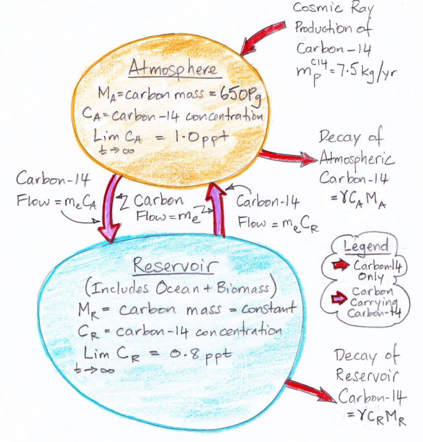
Suppose human beings start to add carbon to our natural, equilibrium atmosphere at a rate mF by burning fossil fuels. We will express mF in petagrams of carbon per year, or Pg/yr. Note that we have been working with carbon masses, not CO2 masses, but we can convert atmospheric carbon mass to atmospheric CO2 mass simply by multiplying by 3.7, which is the ratio of the molar mass of CO2 to the atomic mass of carbon-12. With the addition of mF, our carbon cycle now looks like the diagram below. The time t = 0 yr is the moment just before we start we start adding mF to the atmosphere.
Or, expressed as two differential equations, it looks like this:
We can solve these differential equations in the same way we already solved those of carbon-14 concentration. Examining the equations, we see that we can obtain the behavior of non-radioactive carbon by setting the decay constant, γ, to zero and inserting the the human emission of carbon in place of the cosmic ray creation of carbon-14. More convenient than the analytic solution for our purposes, however, is a numerical solution that we can implement in a spreadsheet and combine with the historical and projected values for mF as our study progresses.
In the numerical solution, we pick a time step small enough that changes in the masses and transfer rates are negligible during the step. Suppose our step is δt. Provided δt is small enough, we can assume, for example, that mA during each step is equal to kA times the value of MA at the beginning of the step. We do not have to account for the fact that MA may be changing during the step, because the time step is so small these changes will be negligible compared to MA. For our carbon cycle, it turns out that one year is always a small enough time step, and in long, slow developments, ten years is small enough.
The following equations are the numerical equivalents of our differential equations. They show how we calculate MA and MR at time t+δt using their values at time t.
The current rate at which humans emit carbon by burning fossil fuels is close to, 10 Pg/yr. In our next post, we will set mF to a constant 10 Pg/yr and calculate how our natural, equilibrium atmosphere responds over ten thousand years.
PS. If you find our carbon cycle drawing too confusing and drab, you can try this one drawn by my youngest son.
Thursday, December 17, 2015
Carbon Cycle: Rate of Transfer
Our study of the radioactive isotope carbon-14, which we began in Carbon-14: Origins and Reservoir, led us to the conclusion that roughly one in every eighteen atmospheric carbon atoms are absorbed by a vast oceanic reservoir each year. When the atmosphere and the reservoir are in equilibrium, the same amount of carbon flows out of the reservoir as into it, so that the mass of carbon in the atmosphere remains constant. But the oceanic reservoir contains over one hundred times as much carbon as the atmosphere.
We now embark upon a series of posts in which we calculate the effect of mankind's carbon emissions upon the atmospheric CO2 concentration. Our starting point for these calculations will be the natural, equilibrium atmosphere and oceans of the late nineteenth century. This atmosphere contains 300 ppmv CO2, which implies a total atmospheric carbon mass of 650 Pg (see here). The oceanic reservoir contains 77,000 Pg, and each year 37 Pg of carbon is exchanged between the atmosphere and the reservoir (see here).
As we showed in our previous post, the probability of an atmospheric carbon atom being transferred into the oceanic reservoir is independent of the number of carbon atoms in the atmosphere. The number of carbon atoms moving into the reservoir is equal to the total number of carbon atoms in the atmosphere divided by eighteen. If we have twice as many carbon atoms, the rate at which they move into the oceanic reservoir will double. If mA is the mass of carbon moving into the reservoir every year, and MA is the mass of carbon in the atmosphere, we must have:
mA = kAMA, where kA = 37 Pg/yr ÷ 650 Pg = 0.057 Pg/yr/Pg.
The probability of a carbon atom in the oceanic reservoir being released into the atmosphere is likewise independent of the number of carbon atoms in the reservoir. If mR is the mass of carbon leaving the reservoir every year and MR is the mass of carbon in the reservoir, we must have:
mR = kRMR, where kR = 37 Pg/yr ÷ 77,000 Pg = 0.00048 Pg/yr/Pg.
If we were to double suddenly the mass of carbon in the atmosphere, carbon would start to move into the oceanic reservoir at double the rate. The graph of atmospheric carbon dioxide concentration would look almost exactly like the graph of carbon-14 concentration after the nuclear bomb tests, which we present here. The movement of carbon between the atmosphere and the oceanic reservoir is governed by almost exactly the same equations as the movement of carbon-14. The only difference is that carbon-14 decays, while carbon-12 lasts forever.
UPDATE: The above calculations are consistent with Henry's Law of gasses dissolving in liquids. Henry's Law applies when the concentration of gas in the liquid has reached equilibrium at a particular temperature with the concentration of gas above the liquid. At equilibrium, the rate at which the liquid emits the gas is equal to the rate at which the liquid absorbs the gas. Henry's Law states that the equilibrium concentration of the gas in the liquid at a particular temperature is proportional to the partial pressure of the gas above the liquid. According to Boyle's Law, the partial pressure of a gas at a particular temperature is proportional to the number of gas molecules per unit volume. In our rate of transfer equations, the rate at which CO2 is absorbed by the ocean is proportional to the concentration of CO2 in the atmosphere, and the rate at which CO2 is emitted is proportional to the concentration in the liquid. If we double the concentration of CO2 in the atmosphere, our equations tell us that the rate of emission by the oceans will equal the rate of absorption only if the concentration of CO2 in the oceans also doubles, which is precisely what Henry's Law requires. Of course, we have not yet considered how changing the temperature of the atmosphere and ocean will affect the rates of transfer, but we will get to that later.
Wednesday, December 9, 2015
Carbon-14: Probability of Exchange
In the carbon cycle of our natural, equilibrium atmosphere, each carbon atom in the atmosphere has a certain probability each year of being absorbed by the reservoir. We call this the probability of exchange in the atmosphere. According to our calculations, 37 Pg of carbon is absorbed by the reservoir each year. Meanwhile, the total mass of carbon in the atmosphere is 650 Pg. To the first approximation, the probability of exchange in the atmosphere is 5.7% per year.
Likewise, a carbon atom in the reservoir has a probability of being released into the atmosphere each year. We have 37 Pg of carbon emerging from the reservoir each year, and the reservoir contains 77,000 Pg of carbon, so the probability of exchange for the reservoir is 0.048% per year.
Almost all carbon in the atmosphere is bound up in CO2. In our previous post we showed that the reservoir is the deep ocean. When a carbon atom enters the deep ocean, it does so as part of a CO2 molecule. The CO2 molecule arrives by chance at the ocean surface, and by further chance it dissolves into the salty water. The CO2 molecule turns into some kind of carbonate ion. This ion mixes down through the top thousand meters of water until it reaches the deep ocean. The carbon atom is now part of the reservoir. The probability of this happening each year is 5.7% for each and every CO2 molecule in the atmosphere.
Likewise, the probability of any carbon atom in the reservoir emerging into the atmosphere as part of a new CO2 molecule each year is 0.048%. The molecule or ion containing the carbon atom mixes up through the top one thousand meters of the ocean, arrives by chance at the surface, and by further chance emerges from the surface as an atmospheric CO2 molecule. (See UPDATE below for discussion of ocean chemistry.)
The exchange of carbon between the atmosphere and the ocean is a first-order chemical process. During the process, each carbon atom is acting alone. It does not require the cooperation of any catalyst to permit it to be dissolved in saltwater or released from saltwater. If we were to double the number of CO2 molecules in the atmosphere, so that six hundred out of every million air molecules were CO2 instead of only three hundred, the probability of any one of them being absorbed by the reservoir each year would remain the same.
If the reservoir were something more complex than the ocean, such as a forest, we would be unable to assert that the probability of exchange was unaffected by the number of CO2 molecules in the atmosphere. A forest needs water and sunlight to convert CO2 into sugar and oxygen. If we double the number of CO2 molecules in the atmosphere, we might find that CO2 molecules are lining up inside forest leaves waiting for enough water and sunlight to arrive before they are turned into plant matter. But our reservoir is the ocean, and entering and leaving it is a statistical process in which each carbon atom acts in isolation.
So far, we have assumed that the atmosphere and reservoir are staying at the same temperature. They could be at different temperatures, but they are neither warming nor cooling. But we note that the probability of exchange is strongly affected by temperature. We have only to look at the decreasing solubility of CO2 in water with temperature, as presented here, to see that this strong effect must exist.
For now, we assume our natural, equilibrium atmosphere, and its carbon reservoir, are neither cooling nor warming. The probability of exchange in the atmosphere remains constant at 5.7% per year, even if we halve or double the atmosphere's CO2 concentration. The probability of exchange in the reservoir remains constant at 0.048% per year, even if the mass of carbon in the reservoir halves or doubles. The probability of exchange is independent of concentration.
This concludes our series of posts on carbon-14. In our upcoming posts, we will apply what carbon-14 has taught us about the Earth's carbon cycle to predict how human CO2 emissions will affect the CO2 concentration of the atmosphere.
UPDATE [08-NOV-16]: In many gas-liquid systems, changes in concentration or acidity can change the probability of emission for a dissolved gas molecule. This variation in probability is possible when the dissolved gas appears as several species in the liquid, some of which cannot emit a gas molecule, while others can. When the relative concentrations of these species changes, the probability of a dissolved gas molecule being emitted also changes. For example, if a gas dissolves into two species A and B in equal proportion, and A has a 10% per year probability of emission while B has a 0% probability, the average probability is 5% per year. If we add acid to the system and the ratio of the two becomes 75% A and 25% B, the probability of emission for each species remains the same, but the average probability rises to 7.5% per year. Our carbon-cycle model is based upon the assumption that the atmosphere-ocean system does not exhibit concentration-dependent nor acidity-dependent probability of emission. Let us justify our assumption with a brief discussion of ocean chemistry.
The top layer of the ocean is saturated with calcium carbonate (CaCO3). The CaCO3 co-exists with the carbonate ions created by CO2 dissolved in water. In Figure 5.6 of Carbonate Equilibria we see the pH of a liquid saturated with calcium carbonate is around 8.5 (log of the H+ concentration is −8.5) for CO2 partial pressure of 300 ppmv (log of CO2 partial pressure is −3.5). The pH of our contemporary ocean is around 8.2, while the pH of a system of only CO2 and water is around 5.8. Continuing with Figure 5.6, for CO2 partial pressures in the range 100 ppmv to 10,000 ppmv (log of CO2 partial pressure is −4 to −2) the carbon content of the solution is dominated by HCO3−. The concentration of HCO3− increases in proportion to the partial pressure of CO2 (its slope is 1.0 in the log-log plot). The concentration of HCO3− is 2.0 times that of Ca2+ throughout the range 100 ppmv to 10,000 ppmv (see Table 5.1 Case 2 for numerical values). As we increase the partial pressure of CO2, an equal number of of CaCO3 and CO2 molecules dissolve. Each CaCO3 molecule that dissolves adds one Ca2+ ion, one HCO3− ion, and one OH− ion to the solution. Each CO2 molecule that dissolves contributes one HCO3− ion and one H+ ion. The OH− and H+ ions combine to form H2O, leaving the other ions in solution. The HCO3− concentration, the dissolved CO2 concentration, and the dissolved CaCO3 concentration all increase in proportion to the partial pressure of CO2. As seawater changes temperature and pressure, the saturation concentration of CaCO3 changes, and CaCO3 can precipitate, as it does in the Persian Gulf, staining the water white.
When a gas and liquid are at equilibrium, there is as much gas entering the liquid per unit time as there is leaving it. Because gaseous CO2 has only one species, its probability of absorption into the ocean does not vary with its concentration. When we double the concentration of atmospheric CO2 from 300 ppmv to 600 ppmv, we double the rate at which it enters the ocean. When the ocean attains a new equilibrium with the 600-ppmv CO2 atmosphere, the rate at which CO2 is emitted by the ocean must be double the rate for 300 ppmv. At the same time, using the CaCO3-CO2-water system as our guide, we see that the concentration of dissolved CO2 will double for this doubling of atmospheric concentration. The doubling of dissolved concentration combined with the doubling of emission tells us that the probability of emission for CO2 molecules in the ocean is constant from 300 ppmv to 600 ppmv.
Another way to model the atmosphere-ocean system is to ignore the calcium carbonate and instead use a CO2-water system with added OH−, such as might come from mixing NaOH with the water. We add OH− in order to increase the pH of the system from 5.8, which applies to the CO2-water system alone, to 8.2, which applies to the ocean. This OH-CO2-water system exhibits more complex behavior in the range 100 ppmv to 1000 ppmv than the CaCO3-CO2-water system. The dissolved CO2 concentration does not increase in proportion to the atmospheric concentration. So far as we can tell, this OH-CO2-water model is what climate scientists are using when they conclude that the ocean will not absorb our CO2 emissions in proportion to atmospheric CO2 concentration. They express its non-linear behavior with a number they call the Revelle Factor. We do not understand why they prefer an OH-CO2-water model to the CaCO3-CO2-water model, nor have we seen in the climate science literature any plots like those of Figure 5.4 or Figure 5.6 for an OH-CO2-water system. The closest we have seen any promoter of the Revelle Factor come to plotting such graphs is here, but that author had no explanation for why they used the OH-CO2-water system instead of the CaCO3-CO2-water system.
Subscribe to:
Posts (Atom)
