The anthropogenic global warming (AGW) hypothesis presented by the majority of today's climatologists has two parts. First it claims that the world is getting exceptionally warm, and second it claims that human carbon dioxide (CO2) emissions are the cause of this warming. Seven years ago, we began our personal investigation of this hypothesis, and we did so by considering whether or not the world was indeed getting exceptionally warm.
The first thing we did was estimate the uncertainty inherent in the measurements of global surface temperature. We concluded that natural variations in local climate introduce an error of roughly 0.14°C in the measurement of the change in temperature between any two points in time. The fact that the error is constant with the time over which we measure the change is a consequence of the particular characteristics of local climate fluctuations.
We downloaded the weather station data from NCDC and calculated the global surface anomaly using a method we called integrated derivatives, but which others have called first differences. The graph we obtained was almost identical to the one obtained by CRU using their complex reference grid method. It remains a mystery to us why institutions like CRU, NASA, and NCDC use such a complex method when a far simpler one will do. All graphs show roughly a 0.6°C rise in global surface temperature from 1950 to 2000. This rise is significant compared to our expected resolution of 0.14°C.
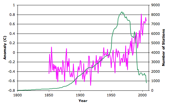
We made this plot superimposing the number of weather stations and the global surface anomaly versus time. The number of weather stations drops dramatically from 1960 and 1990. Only one in four remain active at the end of this thirty-year period. During the same period, the global surface anomaly shows a 0.6°C rise. By selecting subsets of the weather stations, we found that the apparent warming from 1950 to 1990 varied from 0.3°C to 1.0°C depending upon whether we used stations that disappeared in that period, persisted through that period, or existed shorter or longer intervals in the same century. Thus is seemed to us that some significant amount of work would have to be done to eliminate the change in the number of weather stations as a source of error in the data. But we saw no mention whatsoever of this source of error in published papers in which the global surface anomaly is presented, such as Jones et al..
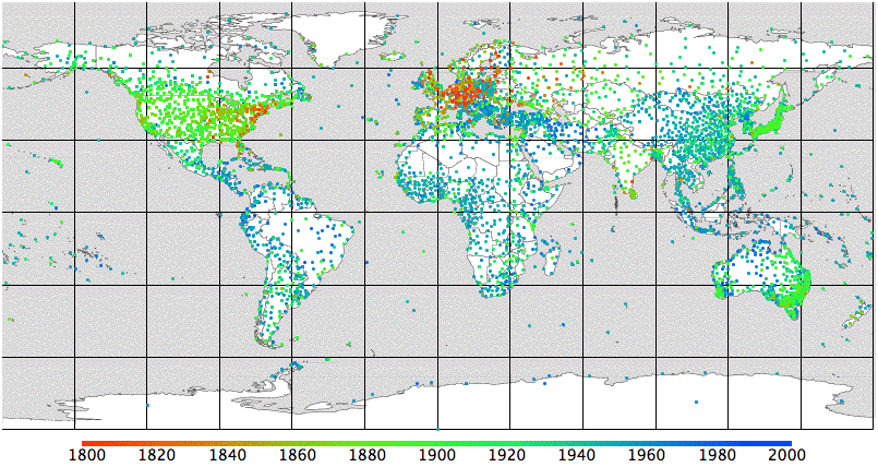
We plotted a global map of the available weather stations, color-coded to show the date they first started reporting. The map shows that almost all stations in the tropics began operating after 1930, while most of those in the temperate regions were operating by 1880. This seems to us to be another source of systematic error in our measurement of the global surface anomaly.
Weather stations might also be affected by the appearance of buildings, tarmac, and road traffic. We found examples of weather stations in which such urban heating caused an apparent warming of several degrees centigrade over a few decades. It seemed to us that this effect would have to be examined in depth by any paper presenting a global surface trend. But papers such as Jones et al. do not address the urban heating issue directly. Instead, they claim that the effect is negligible and refer to other papers as proof. But when we looked up those other papers, we did not find any such proof.
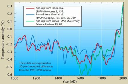
In order to argue that modern temperatures were exceptionally warm, climatologists produced the hockey stick graph, in which a collection of potential long-term measurements of global surface temperature were combined together under the assumption that they could be trusted only to the extent that they showed a temperatures increase from 1950 to 2000. Indeed, if a measurement showed a temperature decline in that period, the hockey stick method would flip the trend over and add it to the combination so that it now contributed to a rise in the same period.
The hockey-stick graph shows no sign of the Medieval Warm Period, in which Greenland was inhabited by farmers, nor the Little Ice Age, when the Thames was known to freeze over, and nor should we expect it to. Given a random set of measurements, the hockey-stick combination method will almost always produce a graph that shows a sharp rise from 1950 to 2000 and a gentle descent during the thousand years before-hand. When applied to the existing measurements of temperature by tree rings, ice cores, and other such indirect methods, it is no surprise that the method produced that same shape.
We presented our doubts about the surface temperature measurements and the hockey stick graph to believers in the AGW hypothesis. We were received with disdain and given no satisfactory answers. Furthermore, the Climategate affair revealed several significant breaches of scientific method by the climate science community. For example, in this graph produced by climatologists for the World Health Organization, the authors removed the tree ring temperature data from 1960 onwards because it showed a decline in temperature, and substituted temperature station measurements in their place. They plotted the combination as a single line. When I asked a prominent climatologists what exactly had been done, he said, "The smooth was calculated using instrumental data past 1960." He declared that a better way to handle the divergence of the tree-ring data from the station measurements would be to cut short the graph of tree-ring data at 1960, so as to hide the decline in temperatures measured by the tree rings.
What we see here is the assumption by climatologists that the world has been warming up and that the global temperature measured by weather stations is correct. This assumption leads them to delete conflicting data on the grounds that it must be bad data. Thus it becomes impossible for them to discover that their assumption is incorrect. By this time, we were skeptical of the global surface anomaly we obtained from the station data. We were no longer certain that the data itself had not been modified by NCDC. We had little reason to trust any other measurement produced by climatologists, we were unimpressed with the hockey-stick method of combining measurements, and we were quite certain that recent temperatures were not exceptional for the past ten thousand years.
We turned our attention to the second part of the AGW hypothesis: the one that says doubling the atmosphere's CO2 concentration will increase the surface temperature by roughly 3°C. It took us a long time to come to a conclusion on this one. The climate models upon which such predictions are based are private property of various climatologists. In any event, we do not trust models produced by a community that is willing to delete data that conflict with its assumptions. If they are willing to delete data, we must assume that they are willing to adjust their models until the models give predictions consistent with their AGW hypothesis.
We began with some laboratory experiments on radiation. We stated the principle of the greenhouse effect. After a great deal of searching around, we eventually obtained the absorption spectrum of various layers of the Earth's atmosphere. This allowed us to confirm that, if the skies remained clear, a doubling of CO2 concentration would cause the world to warm up by about 1.5°C.
But of course the skies don't remain clear. The formation of clouds is a strong function of surface temperature. If the world warms up, there will be more clouds. They will reflect more of the Sun's light, while at the same time, slowing down the radiation of heat into space by the Earth. To determine how these two effects would interact, we built our own climate model, which we called Circulating Cells.
When it comes to determining the effect of increased cloud cover, the most critical parameter to decide upon is the reflection of sunlight by clouds per millimeter of water depth in the cloud. It seemed to us that there should be a large body of literature written recently upon this subject because it is so important to climate modeling. The best paper we found upon the subject was written in 1948, Reflection, Absorption, and Transmission of Insolation by Stratus Cloud. We found a couple of more recent papers about reflection, such as this one, but they do not attempt to provide an empirical formula for the reflection of clouds with increasing cloud depth. We concluded that climatologists are not examining this issue in detail.
In a long sequence of small steps, we built up our climate model until it implemented surface convection, surface heat capacity, evaporation, cloud formation, precipitation, and radiation by clouds. We tested every aspect of the simulation in detail, and based its operating parameters upon our own estimates and upon whatever measurements we could find in climate science journals. We did not choose our model parameters to suit any hypothesis of our own, nor could we have done, because we did not have a model capable of testing the AGW hypothesis until the final stage, and we did not change the parameters in that final stage.
The latest version of our climate model shows that cloud cover increases rapidly as the surface warms above the freezing point of water. The evaporation rate of water from the surface increases approximately as the square of the temperature above freezing, and the only way for water to return to the surface is to form a cloud first. If we ignore the increased reflection of sunlight due to increasing cloud cover, and consider only the slowing-down of radiation into space by the same increase in cloud cover, our model shows roughly 3°C of warming due to a doubling in CO2 concentration. But when we take account of the increased reflection of sunlight by the increasing cloud cover, the warming drops to 0.9°C.
It seems to us that the climate models used by climatologists ignore the reflection of sunlight due to clouds. They may allow for some fixed fraction of sunlight to be reflected by clouds, but they do not allow this fraction to increase with increasing surface temperature. Thus they conclude that the warming due to CO2 doubling will be 3°C. If they took account of the increased reflection, the effect would be far smaller and less dramatic: roughly 1°C.
Doubling the CO2 concentration of the atmosphere will indeed encourage the world to warm up, but not by enough that we should worry. Right now CO2 concentration has increased from roughly 300 ppm to 400 ppm in the past century. If it gets to 600 ppm then we can say that the rise in CO2 concentration will tend to warm the Earth by 1°C. But we are unlikely to be able to check our calculations, because the natural variation in the Earth's climate is itself of order ±1°C from one century to the next.
And so we find ourselves at the end of our journey. Modern warming is not exceptional, and doubling the CO2 concentration will cause the world to warm up by roughly 1°C, not 3°C. The only part of the AGW theory we have not investigated is its assertion that human CO2 emissions are responsible for the increase in atmospheric CO2 concentration over the past century.
My thanks to those of you who took part in the effort, both by private e-mails and in the comments. I would not have continued the effort without your participation. I hope it is clear that my use of "we" instead of "I" is in recognition of the fact that this has been a group effort. I will continue to answer comments on this site, and I will consider any suggestions of further work. To the first approximation, however: we're done.
Subscribe to:
Post Comments (Atom)

My friend Matt writes with the following question. "I really enjoyed reading that. Did you take into account increases in temperature due to an increase in water vapor? More clouds must mean a significant increase in water vapor and as I understand it, water vapor is a much more potent green house gas than carbon dioxide."
ReplyDeleteThat's a good question.
ReplyDeleteNo, we did not simulate the absorption and emission of long-wave radiation by water vapor, because this effect is negligible. We simulated the effect of clouds formed from water vapor, which is two orders of magnitude larger than the effect of water vapor alone.
I recently read somewhere that "95% of the greenhouse effect is due to water vapor." Until now, we have not plotted water vapor depth versus temperature, only cloud depth. At the following link you will find a new graph I made from saved simulation data. It shows the equivalent depth of water vapor in our simulated atmosphere, increasing with surface temperature.
http://www.hashemifamily.com/Kevan/Climate/WVI_1.gif
If the world warms up by 1°C from 288 K to 289 K, we see that water vapor depth will increase by approximately 0.4 mm, or 7%. In the following post you will see the absorption of water vapor and CO2 for the first 3 km of typical temperate, clear-sky atmosphere.
http://homeclimateanalysis.blogspot.com/2010/07/surface-layer.html
If we double CO2 concentration, this doubling has a far greater effect upon the clear-sky atmosphere than a 7% increase in water vapor concentration, so we can safely ignore the increasing absorption and emission of the water vapor itself.
But we cannot ignore the effect of clouds, which become more common when we have more water vapor. It may be that when people say that 95% of the greenhouse effect is due to water vapor, they are in fact talking about the clouds that result from water vapor. I'm not sure.
Anyway: that's why we did not bother to have the long-wave absorption of our atmospheric gas change with temperature.
Peter Newnam writes:
ReplyDeleteDear Kevan,
"We concluded that the resolution of the trend measurement is roughly 0.14°C over any time period."
Given that in one of your responses in your post on “Trends and Noise” you confined the period from the LIA to now:
Perhaps I was unclear about the time-scale I'm considering. I'm looking at changes over the course of a hundred years. Milankovitch cycles take place over tens of thousands of years.
It may be clearer if you stated that, e.g.:
"We concluded that the resolution of the trend measurement is roughly 0.14°C since the end of the LIA."
These sentences in para 3:
"All trends show roughly a 0.6°C rise in global surface temperature from 1950 to 2000. This rise is significant compared to our expected resolution of 0.14°C/half-century."
I am still having trouble understanding the nature of trends in the context of their resolution, so will need to go bit by bit. You have found that the CRU data points for the last 100 years (or since the end of the LIA) deviate from their trend line by an average of 0.14°C. Is that correct?
Cheers,
Peter
In our consideration of the global surface we looked at the Hadley Central England temperature record, and found that its year-to-year change, decade-to-decade change, and century-to-century change had the same standard deviation if we looked at such intervals taken from the three-hundred year record. This is a property of pink noise. We therefore concluded that the inherent random variability in any one temperature station would introduce an error of roughly 0.7°C in the measurement of a linear trend in temperature, if one such existed. If we combine twenty-five independent locations we get 0.14°C, and we estimate that the rather poor distribution of weather stations in the past three centuries is equivalent to 25 well-distributed stations. So we are left with saying the trend we measure with the global set contains a 0.14°C error over any time period.
ReplyDeleteYour modesty does you credit.
ReplyDeleteI'm wondering how the results might change if you extend "Circulating Cells" to the tropopause and if you increase the rows number of the used array. Of course, using a computing system more powerful.
Michele
A good question. A while back, I ran Circulating Cells with 810 W/m2 incoming solar power (over twice the Earth's average), 20 cells vertically, top pressure 25 kPa and bottom pressure 100 kPa. So the altitude of the array will be roughly 10 km. Here is a picture of what the array looks like after it reaches equilibrium.
ReplyDeletehttp://www.hashemifamily.com/Kevan/Climate/DH_810W.png
Surface air temperature is 314 K, which is 14 K higher than the temperature we obtain with the 5-km array and the same incoming power. As you can see in Thickening Clouds we observe the temperature flatting off at 300 K above 500 W/m2 when the array goes up only to 5 km.
Dear Peter,
ReplyDelete> I don’t understand the significance of the relationship between the CRU
> estimate of a 0.6˚C temperature rise between 1950 and 2000 and an
> estimated error of 0.14˚C that is time-independent.
The 0.14°C error I came up with is an estimate of the trend (change in temperature divided by time) we would measure by a least-squares stright-line fit to the data if there were no underlying trend at all. Imagine that the average global temperature is the same every year. Suppose we pick a thousand spots on the world and measure temperature at each spot over ten years. For each spot we fit a straight line by least-squares method to its ten years of data. What is the standard deviation of the slopes of these lines?
Judging from the Hadley Weather station, the slopes will have standard deviation 0.7°C. If we combine together 25 of them we obtain a slope with standard deviation 0.7/√25 = 0.14°C. We estimate that the actual distribution of tens, hundreds, then thousands of weather stations, spreading from a small number of nations to cover much of the world, is like having 25 stations, so the intrinsic error in the global weather station trend is around 0.14°C.
So, when we use our global set of weather stations to measure a trend, we know that over the course of 10 years, we measure the actual trend plus an error, and the standard deviation of this error is around 0.14°C. So if we measure a slope of 0°C/decade, we can be 63% certain that the actual trend is within ±0.14°C and 95% certain that the actual trend is within ±0.28°C (properties of normal distributions).
The interesting thing about the Hadley Record, and all other rural, continuous, undisturbed stations, is that when we perform the estimate of trend error for 50-year or 100-year periods, we get the same answer: 0.7°C is the resolution of our trend measurement over any period at one station. Thus 0.14°C is the resolution of our trend measurement over any period for 25 stations.
The reason the error in trend measurement is constant with the period over which we measure the trend is because the local variations in climate are correlated from one year to the next. (The spectrum of the variations is "pink", or "1/f".) If the local variation were random and independent each year, our trend error would decrease with time period: four times longer, half the error is what we would see.
When you sent me graphs of trends drawn onto the global 300-year record, you drew lines from the temperature at, say 1850 to 2000. Our errors do not apply to lines drawn in that way. They apply to a line fitted to the data so as to minimize the sum of squares of the differences between the data and the line, which is our least squares fit.
The relationship between the 0.6°C rise from 1950 to 2000 and our 0.14°C estimate in trend error is as follows. If we fit a straight line to the global surface anomaly from 1950 to 2000 we get a slope of 0.6°C/half-century. From local climate variation alone, and the poor distribution of the weather stations, we know that this trend measurement contains a stochastic error of 0.14°C/half-century. Thus we are 95% certain that the actual trend is within ±0.28°C of 0.6°C over that half-century.
Of course, we are considering the trend error that arises from local climate variation only. We are not considering systematic errors such as urban heating. The systematic urban heating error would be one that was shared by most weather stations that disappeared from 1950 to 2000, so it is almost impossible to remove it from the data.
Does that answer your question?
Yours, Kevan
Thanks, Kevan, the 2nd last para clarified it for me.
DeleteCheers,
Peter
From Peter Newnam by E-Mail:
ReplyDeleteDear Kevan,
In preparing a printed copy of “Conclusion” for my professor friend, I came across a couple of minor errors:
2nd Para.
The first thing we did was estimate the uncertainty inherent in the measurements [of] global surface temperature.
8th Para.
The hockey-stick graph shows no sign of the Medieval Warm Period, in which Greenland was inhabited by farmers, nor the Little Ice Age, when the Thames froze over every year, and nor should we expect it to.
According to Wikipedia http://en.wikipedia.org/wiki/River_Thames_frost_fairs “Years when the Thames froze” - from 1400 into the 19th century, there were 24 winters in which the Thames was recorded to have frozen over at London; if "more or less frozen over" years (in parentheses) are included, the number is 26: 1408, 1435, 1506, 1514, 1537, 1565, 1595, 1608, 1621, 1635, 1649, 1655, 1663, 1666, 1677, 1684, 1695, 1709, 1716, 1740, (1768), 1776, (1785), 1788, 1795, and 1814.[20]
Cheers,
Peter
Thank you. I corrected the text to say "Thames was known to freeze over". I had been convinced that the Thames froze over every year in the sixteenth century. I think I may have received that impression from paintings of the time, showing people skating around on the ice. But those paintings may have been motivated by a desire to preserve the image of an extraordinarily cold winter, rather than as an example of an annual event.
ReplyDeletePete Newnam sends me a link to the following talk by David Evans, a fellow Electrical Engineer, in which he lists the failure of climate model predictions. In particular, the prediction that the first thing that will happen when the Earth's surface warms up due to CO2 is that it will radiate less heat.
ReplyDeletehttp://www.youtube.com/watch?v=plr-hTRQ2_c&feature=youtu.be
Whatever the predictions by the climate models, they are all wrong according to Evans.
Hi Kevan,
ReplyDelete1. As CO2 is relatively heavy, does it's relative concentration fall off with altitude? (I guess that doubling the concentration of CO2 would double the concentration at each altitude anyhow).
2. Have you included Earth's radioactivity as a source of heat? Would the inclusion of this reduce the necessary greenhouse component?
3. Even without any water & clouds in the atmosphere, wouldn't the extra CO2 which captures more signature radiation cause convective heating of neighboring N2 and O2 which then radiates away more infrared window radiation providing a dampening effect?
Dear Richiebogie,
ReplyDelete(1) The gases in air mix completely. There is no tendency for the heavier molecules to sink. The mixing ratio of CO2 with N2 changes only slightly with altitude.
(2) The Earth's radioactivity is unaffected by atmospheric CO2, so we did not include it in our estimate of the effect of doubling the CO2 concentration. Furthermore, this radioactive heating is less than 1% of Solar heating, so far as we can tell.
(3) These gases are completely mixed. They form a new gas called "air". The absorption spectrum of air is the sum of the absorption spectra of its components gases. Because N2 and O2 are transparent to visible and infra-red light, they don't radiate heat. So I think the answer is "No".
Yours, Kevan
Thanks Kevan. Just on point 3), while N2 and O2 do not have vibrational signature radiation absorption and emission spectra like CO2 and H2O, doesn't all matter emit blackbody spectrum radiation from time to time due to its temperature? ie. collisional energy of N2 converts to energised electrons converts to photons or some process like this?
DeleteAs we show in Radiative Symmetry, a perfectly transparent object emits no thermal radiation. N2 and O2 are almost perfectly transparent in the visible and infrared. They have no means of absorbing a photon of these wavelengths. Likewise, they have no means of emitting a photon of these wavelengths. The absorption of a photon is simply the reverse of the emission of a photon. If absorption is impossible, so is emission. So I think the answer to your question is "No".
DeleteThanks again. I see now that N2 and O2 cannot release window Infrared Radiation, otherwise there wouldn't be a window! To get the full blackbody spectrum you need lots of different elements and molecules. Indeed 'blackbody' means it can absorb and emit all wavelengths.
DeletePerhaps N2 and O2 would emit extra visual and ultraviolet radiation if they become slightly hotter from collisions with excited CO2. However these extra emissions could go out to space or back towards Earth causing warming, as could the extra CO2 signature emissions.
4. Near the top of your Climate Analysis essay, your graph for "Number of Weather Stations Available" seems to have the wrong scale on the right vertical axis.
ReplyDeleteIt seems to peak at around 8200 weather stations in 1970, whereas your text says it peaks at 1700 in 1950.
Dear Richiebogie, Thank you for pointing out that error. It is the text that is wrong, not the graph. I corrected the text to say "peak of 8200 in 1970". Yours, Kevan
ReplyDeleteExamination of this graph:
ReplyDeletehttp://www.aerospaceweb.org/question/atmosphere/atmosphere/layers.gif
suggests that radiation to space in the Troposphere is due to H2O, and radiation to space in the Mesosphere is due to CO2.
As pressure at the mesopause drops so quickly with altitude, doubling CO2 will only raise the mesopause slightly.
Since CO2 has already absorbed all of the available radiation it can absorb, I doubt whether it can make even 1 degree of warming at the surface.
I'm not sure what you mean by "CO2 has already absorbed all of the available radiation it can absorb". Please explain.
DeleteIt is true that H2O is the biggest absorber and emitter of long-wave radiation in the atmosphere. Nevertheless, the absorption and emission by CO2 around wavelength 15 μm is always significant. See here.
Near the Tropopause, we have 2 greenhouse gases. CO2 and H2O.
ReplyDeleteCO2 radiates to H2O or CO2.
H2O radiates to H2O, CO2 and to space.
This means that H2O acts as a radiative drain for CO2.
This is why it is relatively cold.
Near the Stratopause we have 1 greenhouse gas.
CO2 radiates to CO2 only. It is heated by the sun. This is why it is relatively hot.
My interpretation of the graph above:
Near the Mesopause we have 1 greenhouse gas.
Co2 radiates to CO2 or to space. This is why it is relatively cold.
The effect of doubling CO2 concentration may raise the Mesopause and make the Stratopause warmer, but there may not be any temperature change at the Tropopause, as the physics here is determined by the low pressure of H2O.
Why do you believe that CO2 does not radiate into space in the tropopause?
DeleteWhy do you think that CO2 in the stratosphere does not radiate into space?
Why do you think that CO2 and H2O radiate to one another? Their absorption (and therefore their emission) spectra overlap only slightly at around 16 μm, so only a small fraction of what one emits will be absorbed by the other. See here for plots of the absorption spectra of 3-km thick layers of the Earth's atmosphere on a clear day. By the time you get to the tropopause the overlap is insignificant, so that no heat emitted by one will be absorbed by the other.
H2O gives off its radiation at the tropopause because its pressure is so low there. Most of it has fallen out as ice.
DeleteCO2 does not condense at the tropopause. According to Heinz Hug it is such a strong absorber of 15 micron radiation that it can absorb all of the 15 micron radiation coming off the ground in a few metres. It would make sense that its pressure must be very low for it to release any of this radiation to space. The graph I linked to suggests this happens at the mesopause. After I made this observation, I saw that wikipedia says the same about the mesopause. Of course wikipedia is not usually reliable on these topics!
Perhaps you are right about the lack of a radiation overlap between CO2 and H2O vapour, however I believe you explained there is an overlap with CO2 and liquid water and ice which occurs at the tropopause.
However even without the overlap of radiation bands, you have not considered thermalisation of radiation into molecular kinetic energy.
ie. At the stratopause, where the dominant greenhouse gas is CO2, a molecule of CO2 absorbs 15 micron radiation, thermalises it and shares the heat with neighbouring N2, O2 and Ar, making it a locally hot part of the atmosphere.
This works both ways, and so CO2 can use this heat to emit 15 micron radiation and thereby cool neighbouring N2, O2 and Ar. This is noticeable at the mesopause.
However in the troposphere, H2O is the dominant greenhouse gas. CO2 absorbs all available 15 micron radiation coming off the surface, thermalises it and shares the heat with neighbouring N2, O2, Ar and H2O. H2O can then use this heat to emit radiation which is transparent to CO2. In this way, H2O cools the neighbouring N2, O2, Ar and CO2 at the tropopause.
I'm not sure whether any of this affects your 6.6 Watts per Square Metre calculation. It does seem that CO2 is already such a strong absorber, that doubling it's concentration cannot make this much difference. Perhaps like doubling the amount of salt in the ocean...?
When you say "thermalisation of radiation" I think you mean "absorption of radiation" which is always accompanied by an increase in the temperature of the absorbing substance.
DeleteIn our Absorption By All Higher Layers post, and those that preceded it, you will see that we do account for the absorption of radiation by CO2 and H2O, as well as emission by these same components.
It is true that H2O radiates some of the heat absorbed by CO2, but it absorbs more heat from the atmospheric layers lower down, and from the Earth's surface. So the "thermalisation" effect you are thinking about serves only to reduce the amount of warming caused by the greenhouse gases. Their net effect remains one of warming the surface.
Hi Kevan, On further reading, it seems that the ozone layer may be causing some of the warming at the stratopause. Also, your calculation which integrates the spectrum in 0.1 micron chunks seems correct, though I wonder what it would predict going from 330ppm CO2 down to 165ppm down to 82.5ppm down to 41.25... Surely it could not drop the surface temperature by 0.9 degrees celsius every halving... or does it stop dropping once 15 micron radiation is emitted within the tropopause? Can you run your program on 1ppm CO2, or even 1ppb?
ReplyDeleteThank you for your comments.
DeleteI think you may be right about the ozone in the stratosphere. It absorbs UV light and heats up the thin stratospheric atmosphere. I have not simulated the effect, or even performed a crude calculation, so I hesitate to say this is what happens.
If we halve the CO2 from 330 ppm to 165 ppm the surface should cool down, but I don't think it will cool by 0.9°C. First of all, the argument I have heard many times, whereby the CO2 effect is "logarithmic" and therefore every time you halve the concentration you have the same drop in temperature, has no basis I can see at all. It sounds like some kind of hand-waving exercise. Second, the warming in the presence of clouds is more complex, so that we had to run a simulation program rather than calculating directly.
Our simulation program does not implement the CO2 spectrum. You simulate a doubling of CO2 concentration by reducing the transparency fraction by some small amount (I forget by how much).
To obtain the absorption spectrum of the atmosphere for lower CO2 concentrations, such as 30 ppm, I would have to go to the Spectral Calculator site and obtain a whole bunch more plots.
This is a remarkable blog. - congratulations. I have also been on a similar journey through "climate science" over the last couple of years and reached a similar conclusion. You have gone further than me and developed a simple model for radiative transfer and "feedbacks" from water. I will be interested to look through your code.
ReplyDeleteAs you say, AGW is a real effect but will result in only modest warming from a doubling of CO2. The expected warming is only about 1 to 2 maximum degrees C. H2O feedback is negative because otherwise the oceans would have boiled away billions of years ago. The presence of 70% water coverage on Earth regulates temperatures as the sun has brightened over 4 billion years.
A far more serious threat to mankind is the next Ice Age which most likely will gradually begin within 1500 years. By then AGW will seem an insignificant blip.
more information on http://clivebest.com Summary available here
I'm honored by your attention, and glad you liked what you found here. I'll go check your website.
ReplyDelete