Clouds contain microscopic droplets of water. The droplets are around 10 μm in diameter and there are hundreds of them in every cubic centimeter (see here). We discussed the absorption of long-wave radiation by water in an earlier post. We presented a graph of water's absorption length versus radiation wavelength. The graph shows that the absorption length for 5 μm to 60 μm radiation is less than 20 μm. A 100-μm layer of water will absorb 99% of long-wave radiation.
Let us consider the fate of a single long-wave photon as it enters a cloud. The photon may pass all the way through the first centimeter of the cloud without touching a single droplet, or it might strike a droplet. If we assume our droplets have cross-section 100 μm2, the chance of our photon striking any particular droplet while passing through the first cubic centimeter is one in a million. The chance of the photon striking any one of a hundred droplets in the same cubic centimeter is a hundred times greater, or one in ten thousand. In every 100 m of cloud, the expected number of droplets our photon will strike is one (that's one in ten thousand per centimeter times ten thousand centimeters).
When the photon strikes a droplet, it can reflect off the surface or it can enter the liquid. According to this graph from Querry et al., the reflectance of water to long-wave radiation is 2% when the photon approaches at 10° to the perpendicular, 10% at 60°, 20% at 70° and 80% at 87°. The chance of a long-wave photon reflecting from a random spot on the surface of a droplet is around 10%. We also note that most reflection takes place when the photon strikes the droplet at a small angle to the surface, so the photon will continue into the cloud after reflection.
If a photon enters a 10-μm droplet, it will pass through something like 10 μm of water and strike the opposite, inner surface. Here it might reflect back into the droplet. But let's keep things simple: if the photon strikes a droplet, it will most likely enter the droplet, pass through 10 μm of water and keep going.
With 100 droplets in each cubic centimeter, our photon must pass through one droplet on average for each hundred meters of cloud. In 1 km of cloud, our photon will pass through ten droplets. In order to pass through the cloud, it will have to pass through roughly 100 μm of water. But we know that 100 μm of water absorbs 99% of all long-wave radiation. So a 1-km cloud is opaque to long-wave radiation.
Clouds have a different effect upon short-wave radiation, such as sunlight. Short-wave radiation reflects off the air-water surface far more readily than long-wave radiation, and once inside, it is more likely to reflect off the internal surface as well (internal reflection within droplets is what causes rainbows). But on the other hand, the absorption length of visible light in water is tens of meters. The water in a thick cloud will not absorb short-wave radiation. Instead, short-wave radiation changes direction as it encounters water droplets. It can change direction by reflecting off the outer or inner surface of a droplet. It can change direction by refraction as it enters or leaves a droplet. The reason thick clouds are dark is because sunlight is being turned around and re-directed back into space by the cloud's water droplets, not because sunlight is being absorbed by the clouds.
A short-wave photon passing through 1 km of cloud will encounter only ten droplets. These ten droplets are enough to absorb long-wave radiation, but they are not enough to guarantee that the short-wave photon gets re-directed back out of the cloud. With the help of some pencil drawings, we estimate that it would require encounters with one hundred droplets to guarantee that the photon came back out of the cloud on the same side that it went in. A 1-km thick cloud might reflect 10% of the short-wave radiation incident upon it, while a 10-km thick cloud will reflect 90%.
A 1-km layer of cloud acts like a black-body absorber of long-wave radiation. By radiative symmetry, this same 1-km layer must also be a perfect black-body radiator of long-wave radiation. We estimate that this same 1-km of cloud will allow 90% of short-wave radiation to pass through, while reflecting 10%. A 10-km layer of cloud, meanwhile, will allow only 10% of short-wave radiation to pass through, while reflecting 90%.
Heat radiated by the Earth will be absorbed by clouds. These same clouds will radiate their own heat out into space. Sunlight will be reflected off their top surfaces. In our next post, we will consider the effect of a 1-km layer of cloud at altitude 10 km upon the Earth's total escaping power and upon the amount of heat arriving from the Sun.
UPDATE: Cirrus clouds appear to be examples of our 1-km cloud layer. According to NASA, cirrus clouds are opaque to long-wave radiation, but largely transparent to short-wave radiation.
UPDATE: We see here confirmation of our estimates: clouds reflect from 10% to over 90% of short-wave radiation (albedo is 0.1 to over 0.9).
Thursday, October 14, 2010


Thursday, October 7, 2010
Absorption By All Higher Layers
Our Total Escaping Power program calculates the total power radiated by the Earth and its atmosphere given the absorption spectra of a sequence of atmospheric layers. The program does not dictate the thickness of these layers, nor even do the layers have to have the same thickness, but we did assume that radiation passing through one layer will be certain to pass through all higher layers. If we want to experiment with greater water vapor content in an upper layer, or if we want to include a layer of clouds, we will need a program that does not rely upon this assumption.
We modified our TEP1 program to produce TEP2. The new program applies the absorption of all higher layers to upward radiation. The result is a decrease in total escaping power. Here is the output of the new program when we apply it to our EA1 spectra, which assume 330 ppm CO2. We have added by hand a final column giving the change in escaping power caused by applying the absorption of all upper layers.
The enhancement of our model makes only a slight change in our CO2 doubling temperature, but it allows us to include upper layers that are more absorbent than lower layers. We can look forward to including layers of clouds and layers of excess humidity, and seeing how they effect the total escaping power.
We modified our TEP1 program to produce TEP2. The new program applies the absorption of all higher layers to upward radiation. The result is a decrease in total escaping power. Here is the output of the new program when we apply it to our EA1 spectra, which assume 330 ppm CO2. We have added by hand a final column giving the change in escaping power caused by applying the absorption of all upper layers.
---------------------------------------------------------In our discussion of TEP1, we claimed that our assumption of upper transparency would cause less than a 10% error in our calculation of total escaping power. It turns out that including the absorption of upper layers causes a 15% drop. Let's apply TEP1 to our EA2 spectra, which assume 660 ppm CO2.
Name Temp BB Layer Escaping Change
---------------------------------------------------------
Surface 290.0 401.1 388.8 80.0 -9.8
0-km 280.0 348.5 262.6 46.1 -12.8
3-km 270.0 301.3 184.8 39.7 -10.0
6-km 250.0 221.5 111.5 44.6 -6.8
9-km 230.0 158.7 50.7 26.4 -3.0
12-km 220.0 132.8 22.2 10.1 -1.1
15-km 220.0 132.8 14.4 5.5 -0.0
---------------------------------------------------------
Total: 252.5 -43.5
---------------------------------------------------------
------------------------------------------------We see a 5 W/m2 decrease in total escaping power due to doubling the CO2 concentration from 330 ppm to 660 ppm. The drop is 2.0%, slightly less than the 2.2% calculated by TEP1. If we repeat our calculation of CO2 doubling temperature using TEP2, we arrive at a value of 1.5°C, slightly less than the 1.6°C calculated by TEP1.
Name Temp BB Layer Escaping
------------------------------------------------
Surface 290.0 401.1 388.8 78.8
0-km 280.0 348.5 264.0 44.2
3-km 270.0 301.3 188.6 38.2
6-km 250.0 221.5 115.2 43.9
9-km 230.0 158.7 53.4 26.4
12-km 220.0 132.8 24.2 10.3
15-km 220.0 132.8 16.3 5.7
------------------------------------------------
Total: 247.5
------------------------------------------------
The enhancement of our model makes only a slight change in our CO2 doubling temperature, but it allows us to include upper layers that are more absorbent than lower layers. We can look forward to including layers of clouds and layers of excess humidity, and seeing how they effect the total escaping power.
Wednesday, October 6, 2010
With 660 ppm CO2
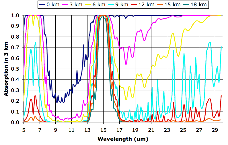
In our In our previous post we extended our atmospheric absorption spectra to cover wavelengths 5 μm to 60 μm. These spectra assume CO2 concentration 330 ppm, which is typical for the Earth today, and temperature and water vapor concentration typical for a 30°N on a clear spring day. We plotted the extended spectra and applied them as input to our total escaping power program. The program says that the total power radiated by the Earth's surface and its atmosphere below the tropopause is 296.0 W.
Today we make one change to our atmospheric conditions: we double the CO2 concentration to 660 ppm. We leave water vapor concentration, temperature, and pressure the same. With the help of the Spectral Calculator, we obtain new absorption spectra and plot them.
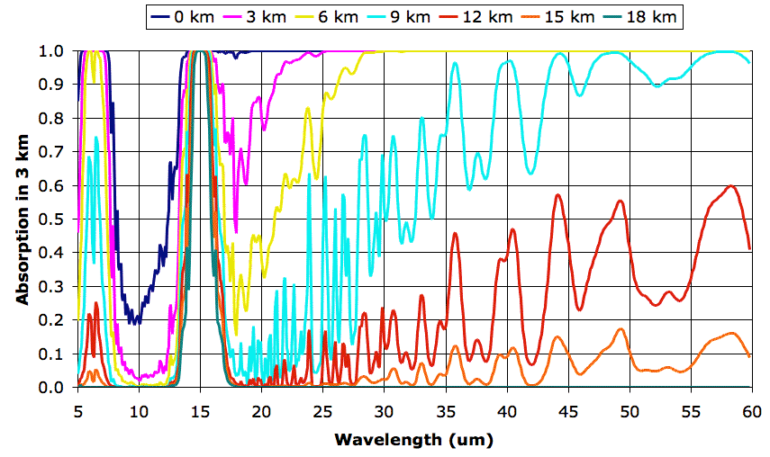
We feed our new spectra into our total escaping power program, and obtain the following output. The final column we added by hand. It gives us the change in total escaping power when we raise CO2 concentration from 330 ppm to 660 ppm.
According to Stephan's Law, the amount of power radiated by a black body increases as the fourth power of its temperature. For small changes in temperature, the amount of power radiated by any body will increase as the fourth power of its temperature. A 1% increase in temperature will cause a 4% increase in radiated power. In order to increase total escaping power by 2.2%, we can increase the temperature of the Earth's surface and all the atmospheric layers by one quarter of 2.2%, or 0.55%. We increased all our layer temperatures by 0.55% and applied our total escaping power program to the resulting atmospheric layers. We obtain the following output. Note that the new temperatures are recorded in the first column.
Our analysis considered only the heat radiated by the troposphere, which is the region of the atmosphere below the tropopause. We ignored the effect of increased CO2 upon the stratosphere, which is the region above the tropopause. Even though there is no net heat flow between the troposphere and the stratosphere, an overall warming or cooling of the stratosphere will affect the temperature of the troposphere, and therefore change its total radiated power. Furthermore, we ignored the effect of increased CO2 upon radiation arriving from the Sun. We will consider these effects in future posts. In our next post, however, we will try doubling the water vapor concentration in various atmospheric layers and re-calculating total escaping power. By this means, we will be able to determine whether the effect of CO2 upon total escaping power is significant compared that of water vapor.
UPDATE: See slightly improved calculation of CO2 warming in next post, where we arrive at 1.5°C instead of 1.6°C as the size of the effect.
Today we make one change to our atmospheric conditions: we double the CO2 concentration to 660 ppm. We leave water vapor concentration, temperature, and pressure the same. With the help of the Spectral Calculator, we obtain new absorption spectra and plot them.
We feed our new spectra into our total escaping power program, and obtain the following output. The final column we added by hand. It gives us the change in total escaping power when we raise CO2 concentration from 330 ppm to 660 ppm.
-------------------------------------------------------The total escaping power drops by 6.6 W/m2. The power escaping from the Earth's surface and the first three 3-km layers of the atmosphere decreases by 7.2 W/m2, but the power radiated by the top three layers increases by 0.8 W/m2. In the lower layers, more CO2 causes more radiation to be absorbed on its way into space. In the upper layers, more CO2 allows the atmosphere to radiate its heat more efficiently into space. We see that the increased absorption far outweighs the increased radiation, and the result is a 2.2% reduction in the heat escaping the Earth.
Name Temp BB Layer Escaping Change
-------------------------------------------------------
Surface 290.0 401.1 388.8 88.2 -1.6
0-km 280.0 348.5 264.0 55.6 -3.3
3-km 270.0 301.3 188.6 47.8 -1.9
6-km 250.0 221.5 115.2 51.0 -0.4
9-km 230.0 158.7 53.4 29.7 +0.3
12-km 220.0 132.8 24.2 11.5 +0.3
15-km 220.0 132.8 16.3 5.7 +0.2
-------------------------------------------------------
Total: 289.4 -6.6
-------------------------------------------------------
According to Stephan's Law, the amount of power radiated by a black body increases as the fourth power of its temperature. For small changes in temperature, the amount of power radiated by any body will increase as the fourth power of its temperature. A 1% increase in temperature will cause a 4% increase in radiated power. In order to increase total escaping power by 2.2%, we can increase the temperature of the Earth's surface and all the atmospheric layers by one quarter of 2.2%, or 0.55%. We increased all our layer temperatures by 0.55% and applied our total escaping power program to the resulting atmospheric layers. We obtain the following output. Note that the new temperatures are recorded in the first column.
------------------------------------------------We see that there is no net change in total radiated power when we combine a doubling of CO2 concentration with a 1.6°C warming of the Earth's surface. That's not to say that the Earth will actually warm up by 1.6°C if we double the CO2 concentration, because the climate might be a chaotic system that defies such simple logic, or a system with feedback that acts in quite the opposite manner to our expectations. Nevertheless, in the absence of such complex behavior, the doubling the CO2 concentration will tend to warm the Earth by 1.6°C. This 1.6°C is our estimate of the Earth's CO2 doubling temperature.
Name Temp BB Layer Escaping
------------------------------------------------
Surface 291.6 410.0 397.5 90.6
0-km 281.5 356.1 269.3 57.0
3-km 271.5 308.1 192.3 48.8
6-km 251.4 226.5 117.4 52.0
9-km 231.3 162.3 54.4 30.2
12-km 221.2 135.8 24.7 11.7
15-km 221.2 135.8 16.7 5.9
------------------------------------------------
Total: 296.1
------------------------------------------------
Our analysis considered only the heat radiated by the troposphere, which is the region of the atmosphere below the tropopause. We ignored the effect of increased CO2 upon the stratosphere, which is the region above the tropopause. Even though there is no net heat flow between the troposphere and the stratosphere, an overall warming or cooling of the stratosphere will affect the temperature of the troposphere, and therefore change its total radiated power. Furthermore, we ignored the effect of increased CO2 upon radiation arriving from the Sun. We will consider these effects in future posts. In our next post, however, we will try doubling the water vapor concentration in various atmospheric layers and re-calculating total escaping power. By this means, we will be able to determine whether the effect of CO2 upon total escaping power is significant compared that of water vapor.
UPDATE: See slightly improved calculation of CO2 warming in next post, where we arrive at 1.5°C instead of 1.6°C as the size of the effect.
Wednesday, September 29, 2010
Extended Atmospheric Absorption Spectra
In our previous post we concluded that we needed to extend our existing absorption spectra to cover the range 5 μm to 60 μm. So we returned to the Spectral Calculator and, entered our gas properties for each atmospheric layer, and obtained the absorption spectra from 30 μm to 60 μm. We added these to our existing spectra and obtained the following graph (click for a larger version).
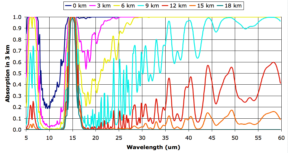
As a point of detail, each spectrum we receive from the Spectral Calculator contain tens of thousands of values. We condense the spectra using a program that calculates the average absorption in each 0.1-μm window. The result is a spectrum with a point every tenth of a micron. You will find the original spectra in our data archive, in the EA_1 folder. You will find the condensed spectra here. The condensed file can act as input to our climate models and is convenient for generating plots like the one above.
We apply our total escaping power program to our extended spectra and obtain the following values for power per square meter. For an explanation of the various columns, see here.
We experiment with the black-body radiation spectrum using this program. When we integrate in 0.1-μm steps all the way from 1 μm to 300 μm, we get a total power of 401.0 W/m2, which is almost exactly what we obtain from Stefan's Law. We use our program to determine the power radiated by a black body at various wavelengths.
Our next step is to generate a new set of spectra for the atmosphere with 660 ppm CO2, and see how the total escaping power changes. Our guess is that the total escaping power will decrease, but we are not sure by how much.
As a point of detail, each spectrum we receive from the Spectral Calculator contain tens of thousands of values. We condense the spectra using a program that calculates the average absorption in each 0.1-μm window. The result is a spectrum with a point every tenth of a micron. You will find the original spectra in our data archive, in the EA_1 folder. You will find the condensed spectra here. The condensed file can act as input to our climate models and is convenient for generating plots like the one above.
We apply our total escaping power program to our extended spectra and obtain the following values for power per square meter. For an explanation of the various columns, see here.
------------------------------------------------Let's look at the first line of numbers, which apply to the surface of the Earth. We treat the surface as a black body, as we justify elsewhere. Using Stefan's Law we find that a black body at 290 K (that's 17°C) should radiate 401.1 W/m2. Our calculator adds the power radiated in each 0.1-μm window from 5 μm to 60 μm, in a process we call numerical integration, and arrives at 388.8 W/m2. That's closer to 401.1 W/m2 than the 349.0 W/m2 we obtained when we our calculation extended only to 30 μm. But we still have a difference of 12.3 W/m2.
Name Temp BB Layer Escaping
------------------------------------------------
Surface 290.0 401.1 388.8 89.8
0-km 280.0 348.5 262.6 58.9
3-km 270.0 301.3 184.8 49.7
6-km 250.0 221.5 111.5 51.4
9-km 230.0 158.7 50.7 29.4
12-km 220.0 132.8 22.2 11.2
15-km 220.0 132.8 14.4 5.5
------------------------------------------------
Total: 296.0
------------------------------------------------
We experiment with the black-body radiation spectrum using this program. When we integrate in 0.1-μm steps all the way from 1 μm to 300 μm, we get a total power of 401.0 W/m2, which is almost exactly what we obtain from Stefan's Law. We use our program to determine the power radiated by a black body at various wavelengths.
--------------------------We have a total of 12.2 W outside the 5-60 μm range of our absorption spectra. In the future, perhaps we will extend our spectra to include this missing 3%, but for now we are content with our omission. Furthermore, we are satisfied that our numerical integration in 0.1-μm steps, which is the basis of our climate model's calculations, is accurate to better than 0.1%.
Range (um) Power (W/m^2)
--------------------------
0.1-1 0.0
1-5 3.8
5-60 388.8
60-100 6.4
100-200 1.8
200-300 0.2
--------------------------
Total 401.0
--------------------------
Our next step is to generate a new set of spectra for the atmosphere with 660 ppm CO2, and see how the total escaping power changes. Our guess is that the total escaping power will decrease, but we are not sure by how much.
Wednesday, September 22, 2010
Total Escaping Power
Our current approach to modeling the Earth's greenhouse effect is to divide the Earth's atmosphere in to 3-km layers. So far, we have considered how each of the first seven layers absorbs and emits long-wave radiation. Our study of these seven layers has been motivated by a desire to calculate the total heat radiated into space by the Earth and its atmosphere, and ultimately to estimate the strength of the relationship between the Earth's surface temperature and the concentration of CO2 in its atmosphere.
In previous posts, we simplified our discussion by assuming that each atmospheric layer was either perfectly transparent or absolutely opaque at each wavelength. This assumption, combined with an examination of the absorption spectra, allowed us to say that all radiation passing through one layer would be sure to pass through all higher layers as well. Furthermore, our assumption allowed us to ignore the fact that most upward radiation is not vertical, but at some angle to the vertical. Radiation traveling at 60° to the vertical will pass through 6 km of air as it ascends through a 3-km layer, and so is more likely to be absorbed by the layer. But if we assume that the 3-km layer is either perfectly transparent or absolutely opaque, we conclude that radiation of a particular wavelength will either pass entirely through the layer or be entirely absorbed by the layer, regardless of its direction of travel.
Today we present our first layered-atmosphere computer model. The model does not assume that each layer is either transparent or opaque. When we calculate the power escaping into space from layer A at temperature T between wavelengths 10.0 μm and 10.1 μm, we proceed as follows. We start with the black-body radiation power density at wavelength 10 μm and temperature T. This power density is almost constant in the narrow range 10.0 μm to 10.1 μm, so we multiply the power density at 10.0 μm by 0.1 μm and obtain a good estimate of the power radiated between 10.0 μm and 10.1 μm. Now we multiply this power by the fractional absorption of layer A at 10.0 μm. The principle of radiative symmetry dictates that the efficiency with which a body emits radiation at a particular wavelength, as a fraction of the power emitted by a black body, is exactly equal to the efficiency with which it absorbs that same wavelength. So we now have the power radiated by layer A between wavelengths 10.0 μm and 10.1 μm. By assumption, whatever is not absorbed by the layer above A will escape into space, so we multiply the power radiated by A by the fractional transmission at 10.0 μm (that's one minus the fractional absorption at 10.0 μm) of the layer immediately above, and so arrive at the power between 10.0-10.1 μm that escapes from layer A into space.
To obtain the total power escaping into space from each layer, we add up the power escaping in all the 0.1-μm bands from 5 μm to 30 μm, which is the extent of our absorption spectra. We will include the surface of the Earth as its own layer. As we have in the past, we will assume the Earth's surface is a black-body radiator. Thus our program will calculate for us the total power escaping from the Earth into space, and allow us to see how much of this power is radiated by the surface and by each atmospheric layer.
Although we have dropped the transparent-opaque simplification, we retain two of its corollaries. First, we ignore the fact that most upward radiation is not vertical. Second, we assume that any radiation that manages to pass through the layer immediately above will be sure to pass through all remaining layers. These assumptions will effect our estimates, but we believe the effect will be less than 10%. In the future we may enhance our model to remove these assumptions, but for now we will start with a simple model.
We wrote our computer model in TclTk. You will find it here. The program takes as its input this file containing the names of the layers, their temperatures, and their absorption spectra. It produces the following output.
We see immediately that the power escaping from the 15-km layer is only 1.5% of the total escaping power, and twenty times less than the power escaping from the Earth's surface. The top three layers of the atmosphere combined contribute less than 10% to the total escaping power. These are the layers in which radiation is dominated by CO2. In the lower layers, radiation is dominated by water vapor.
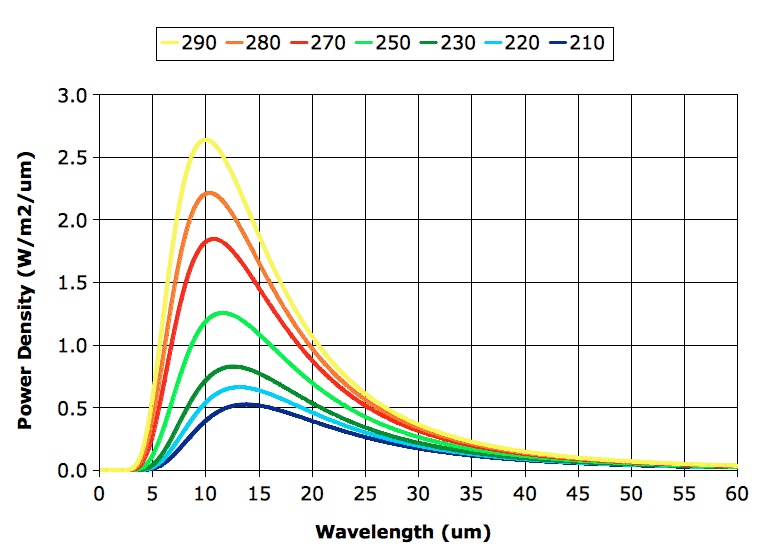
Before we proceed with exercising our model, however, we must correct a deficiency in our existing spectra. Our spectra extend from 5 μm to 30 μm, but it turns out that a significant portion of the heat radiated by the Earth's atmospheric layers is radiated in the range 30 μm to 60 μm, as you can see in the graph below. (In case you are interested, we obtained the curves of this graph using this program.)
The "BB" column in our table gives the power a black body would radiate, as calculated using Stefan's Law. Our calculation assumes the Earth's surface is a black body, so when we see 401 W/m2 in the "BB" column, we expect to see the same value in the "Layer" column. But we don't, and the reason we don't is because our calculation adds up only the power radiated by each layer in the range 5 μm to 30 μm. A black body at 290 K radiates only 349 W/m2 in this range. The remaining 52 W/m2 it radiates in the range 30 μm to 60 μm.
We must go back to the Spectral Calculator and extend our spectra to 60 μm. While we are there, we will obtain the spectra for 660 ppm CO2 and 165 ppm CO2 as well.
In previous posts, we simplified our discussion by assuming that each atmospheric layer was either perfectly transparent or absolutely opaque at each wavelength. This assumption, combined with an examination of the absorption spectra, allowed us to say that all radiation passing through one layer would be sure to pass through all higher layers as well. Furthermore, our assumption allowed us to ignore the fact that most upward radiation is not vertical, but at some angle to the vertical. Radiation traveling at 60° to the vertical will pass through 6 km of air as it ascends through a 3-km layer, and so is more likely to be absorbed by the layer. But if we assume that the 3-km layer is either perfectly transparent or absolutely opaque, we conclude that radiation of a particular wavelength will either pass entirely through the layer or be entirely absorbed by the layer, regardless of its direction of travel.
Today we present our first layered-atmosphere computer model. The model does not assume that each layer is either transparent or opaque. When we calculate the power escaping into space from layer A at temperature T between wavelengths 10.0 μm and 10.1 μm, we proceed as follows. We start with the black-body radiation power density at wavelength 10 μm and temperature T. This power density is almost constant in the narrow range 10.0 μm to 10.1 μm, so we multiply the power density at 10.0 μm by 0.1 μm and obtain a good estimate of the power radiated between 10.0 μm and 10.1 μm. Now we multiply this power by the fractional absorption of layer A at 10.0 μm. The principle of radiative symmetry dictates that the efficiency with which a body emits radiation at a particular wavelength, as a fraction of the power emitted by a black body, is exactly equal to the efficiency with which it absorbs that same wavelength. So we now have the power radiated by layer A between wavelengths 10.0 μm and 10.1 μm. By assumption, whatever is not absorbed by the layer above A will escape into space, so we multiply the power radiated by A by the fractional transmission at 10.0 μm (that's one minus the fractional absorption at 10.0 μm) of the layer immediately above, and so arrive at the power between 10.0-10.1 μm that escapes from layer A into space.
To obtain the total power escaping into space from each layer, we add up the power escaping in all the 0.1-μm bands from 5 μm to 30 μm, which is the extent of our absorption spectra. We will include the surface of the Earth as its own layer. As we have in the past, we will assume the Earth's surface is a black-body radiator. Thus our program will calculate for us the total power escaping from the Earth into space, and allow us to see how much of this power is radiated by the surface and by each atmospheric layer.
Although we have dropped the transparent-opaque simplification, we retain two of its corollaries. First, we ignore the fact that most upward radiation is not vertical. Second, we assume that any radiation that manages to pass through the layer immediately above will be sure to pass through all remaining layers. These assumptions will effect our estimates, but we believe the effect will be less than 10%. In the future we may enhance our model to remove these assumptions, but for now we will start with a simple model.
We wrote our computer model in TclTk. You will find it here. The program takes as its input this file containing the names of the layers, their temperatures, and their absorption spectra. It produces the following output.
------------------------------------------------The "Layer" column is the power radiated upwards by each square meter between 5 μm and 30 μm. The "Escaping" column is the power that escapes. We used 290 K for the surface temperature, which is 17°C. The total power escaping into space is 268 W/m2. We don't have radiation from the 18-km layer, because we use this layer only as an absorber for radiation from the 15-km layer. The atmosphere above 15 km plays little or no part in atmospheric convection because it is above the tropopause.
Name Temp BB Layer Escaping
------------------------------------------------
Surface 290.0 401.1 349.0 89.7
0-km 280.0 348.5 225.3 58.8
3-km 270.0 301.3 150.0 49.8
6-km 250.0 221.5 81.5 44.4
9-km 230.0 158.7 31.2 15.4
12-km 220.0 132.8 16.3 5.8
15-km 220.0 132.8 13.1 4.2
------------------------------------------------
Total: 268.2
------------------------------------------------
We see immediately that the power escaping from the 15-km layer is only 1.5% of the total escaping power, and twenty times less than the power escaping from the Earth's surface. The top three layers of the atmosphere combined contribute less than 10% to the total escaping power. These are the layers in which radiation is dominated by CO2. In the lower layers, radiation is dominated by water vapor.
Before we proceed with exercising our model, however, we must correct a deficiency in our existing spectra. Our spectra extend from 5 μm to 30 μm, but it turns out that a significant portion of the heat radiated by the Earth's atmospheric layers is radiated in the range 30 μm to 60 μm, as you can see in the graph below. (In case you are interested, we obtained the curves of this graph using this program.)
The "BB" column in our table gives the power a black body would radiate, as calculated using Stefan's Law. Our calculation assumes the Earth's surface is a black body, so when we see 401 W/m2 in the "BB" column, we expect to see the same value in the "Layer" column. But we don't, and the reason we don't is because our calculation adds up only the power radiated by each layer in the range 5 μm to 30 μm. A black body at 290 K radiates only 349 W/m2 in this range. The remaining 52 W/m2 it radiates in the range 30 μm to 60 μm.
We must go back to the Spectral Calculator and extend our spectra to 60 μm. While we are there, we will obtain the spectra for 660 ppm CO2 and 165 ppm CO2 as well.
Wednesday, September 15, 2010
CO2 Absorption Band
In our previous post, we presented this graph of absorption by the Earth's atmosphere between 18 km and 21 km. This absorption is due entirely to CO2. In our calculations we set water vapor concentration to zero. Indeed, the absorption in the range 13-17 μm is due almost entirely to CO2 starting at an altitude of 9 km. The following plot gives us a close-up of the CO2 absorption in 3-km layers.
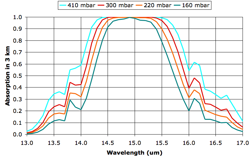
The four graphs are for 9, 12, 15, and 18 km, but we have named them after their atmospheric pressures, 410, 300, 220, and 160 mbar respectively. These pressures do not, in fact, correspond exactly to the pressures we observe in the atmosphere, because our pressure calculation ignores the drop in temperature as we ascend, but we used these pressure values when we calculated the spectra.
What we see between the absorption at 160 mbar and 300 mbar is the effect of doubling the density of CO2 molecules. In both cases, CO2 concentration is 330 ppm, which means 330 out of every 1,000,000 molecules are CO2. But the number of molecules per cubic meter increases approximately with the pressure, so the 300-mbar plot represents twice as much CO2 per cubic meter as the 160-mbar plot.
The absorption at 160 mbar for wavelength 14 μm is 21%, rising to 99% at 15 μm. The absorption at 300 mbar for wavelength 14 μm is 42%, rising to 99% at 15 μm. Twice as much CO2 in a 3-km layer leads to twice as much absorption of 14-μm radiation, but no significant increase in absorption of 15-μm radiation. We are particularly interested in the effect of doubling CO2 concentration, so let us try to get a better idea of how much more absorbing power the atmosphere has at 300 mbar than 160 mbar. Suppose a lower layer of the atmosphere emits uniformly in the band 13-17 μm, so that there is equal power in each 0.5-μm division of our graph. We can count squares under each graph and divide by the total number of squares to get the fraction of power absorbed by CO2 at each pressure. We come up with 43% at 160 mbar and 56% at 300 mbar.
Of course, the lower layers of the atmosphere do not radiate uniformly in the 13-17 μm band. Their radiation in this band is dominated by their own CO2, in accordance with radiative symmetry. The 300-mbar layer will receive radiation from the 410-mbar layer below it, and this radiation will have a power distribution that matches the 410-mbar layer's own absorption spectrum. At 14 μm, for example, the 410-mbar layer will radiate only 60% as much power as it does at 15 μm. In our spreadsheet we multiply the radiation spectrum of the 410-mbar layer by the absorption spectrum of the 300-mbar layer, and find that the 300-mbar layer absorbs 74% of the radiation arriving from the 410-mbar layer below. Meanwhile, the 160-mbar layer absorbs 70% of radiation from the 220-mbar layer below it.
The greenhouse effect causes a convection cycle in the Earth's atmosphere, which transports heat from the Earth's surface to the tropopause. All layers of the Earth's atmosphere up to the tropopause radiate heat out into space through the thinner, upper layers. As our previous posts have shown, radiation by the lower layers is dominated by water vapor, while radiation by the upper layers is dominated by CO2. Our calculations suggest that doubling the atmosphere's CO2 concentration will cause only a slight increase in the absorption and emission of radiation by the upper layers. In future posts, we will try to estimate how much this slight increase in absorption will raise the surface temperature of the Earth.
The four graphs are for 9, 12, 15, and 18 km, but we have named them after their atmospheric pressures, 410, 300, 220, and 160 mbar respectively. These pressures do not, in fact, correspond exactly to the pressures we observe in the atmosphere, because our pressure calculation ignores the drop in temperature as we ascend, but we used these pressure values when we calculated the spectra.
What we see between the absorption at 160 mbar and 300 mbar is the effect of doubling the density of CO2 molecules. In both cases, CO2 concentration is 330 ppm, which means 330 out of every 1,000,000 molecules are CO2. But the number of molecules per cubic meter increases approximately with the pressure, so the 300-mbar plot represents twice as much CO2 per cubic meter as the 160-mbar plot.
The absorption at 160 mbar for wavelength 14 μm is 21%, rising to 99% at 15 μm. The absorption at 300 mbar for wavelength 14 μm is 42%, rising to 99% at 15 μm. Twice as much CO2 in a 3-km layer leads to twice as much absorption of 14-μm radiation, but no significant increase in absorption of 15-μm radiation. We are particularly interested in the effect of doubling CO2 concentration, so let us try to get a better idea of how much more absorbing power the atmosphere has at 300 mbar than 160 mbar. Suppose a lower layer of the atmosphere emits uniformly in the band 13-17 μm, so that there is equal power in each 0.5-μm division of our graph. We can count squares under each graph and divide by the total number of squares to get the fraction of power absorbed by CO2 at each pressure. We come up with 43% at 160 mbar and 56% at 300 mbar.
Of course, the lower layers of the atmosphere do not radiate uniformly in the 13-17 μm band. Their radiation in this band is dominated by their own CO2, in accordance with radiative symmetry. The 300-mbar layer will receive radiation from the 410-mbar layer below it, and this radiation will have a power distribution that matches the 410-mbar layer's own absorption spectrum. At 14 μm, for example, the 410-mbar layer will radiate only 60% as much power as it does at 15 μm. In our spreadsheet we multiply the radiation spectrum of the 410-mbar layer by the absorption spectrum of the 300-mbar layer, and find that the 300-mbar layer absorbs 74% of the radiation arriving from the 410-mbar layer below. Meanwhile, the 160-mbar layer absorbs 70% of radiation from the 220-mbar layer below it.
The greenhouse effect causes a convection cycle in the Earth's atmosphere, which transports heat from the Earth's surface to the tropopause. All layers of the Earth's atmosphere up to the tropopause radiate heat out into space through the thinner, upper layers. As our previous posts have shown, radiation by the lower layers is dominated by water vapor, while radiation by the upper layers is dominated by CO2. Our calculations suggest that doubling the atmosphere's CO2 concentration will cause only a slight increase in the absorption and emission of radiation by the upper layers. In future posts, we will try to estimate how much this slight increase in absorption will raise the surface temperature of the Earth.
Wednesday, September 1, 2010
The Earth's Tropopause
In our previous post, we noted that the temperature of the atmosphere does not drop by more than a few degrees Centigrade between altitude 12 km and 18 km. We concluded that altitude 15 km corresponds roughly to the atmosphere's tropopause, and therefore marks the top of its convection cycle. Today we consider if there is any significant heat transfer between the tropopause and the upper atmosphere.
The following graph shows the absorption of long-wave radiation by the seventh 3-km layer of the Earth's atmosphere, from altitude 18 km to 21 km. This line is the same as the 18-km line in our Earth's Atmosphere post. The absorption is typical of a clear day in April, at latitude 30°N. We assume water vapor content is zero, but CO2 concentration remains 330 ppm. We assume air pressure is 160 mbar and temperature is 210 K, or −63°C.
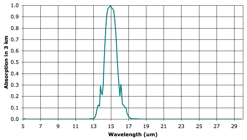
In the seventh layer, absorption by CO2 remains strong. As before, we say our 3-km layer is opaque at a particular wavelength when it absorbs more than 63% of that wavelength, and is transparent otherwise. The seventh 3-km layer is opaque from 14.3 to 15.6 μm, while the sixth layer was opaque to 14.3 to 15.7 μm. The seventh layer will absorb roughly 93% of the heat radiated upwards by the CO2 in the sixth layer.
We note that the actual pressure in the Earth's atmosphere at 18 km is closer to 130 mbar. We calculated atmospheric pressure using our constant-temperature model of atmospheric pressure, and this model starts to be increasingly inaccurate in the cold upper layers of the atmosphere.
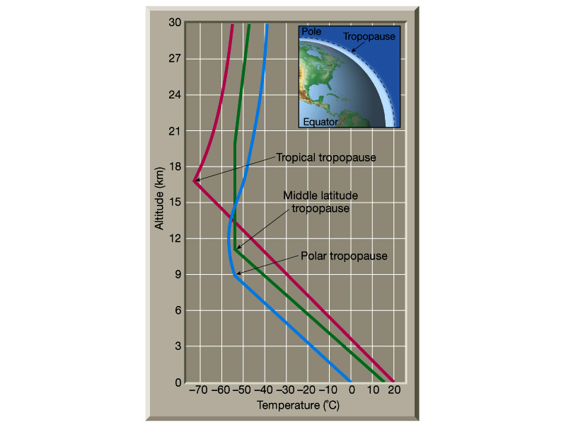
When we chose our temperatures, we were looking at this plot and rounding to the nearest 10 K. If you look at the plot yourself, you will see that the minimum temperature varies with latitude, and that the minimum spreads over a large range. We see this variation with latitude and the extent of the minimum in plots like this one also. In the case of 30°N, the temperature minimum extends from roughly 12 km to 22 km. The tropopause is the altitude at which the temperature stops dropping with pressure as it would in adiabatic expansion. Thus the tropopause is not at the altitude of minimum temperature, but rather at the altitude where temperature stops dropping adiabatically with pressure.
We go back to this plot and estimate the tropopause altitude as 9 km at 90°N (the north pole), 12 km at 30°N, and 13 km at 0°N (the equator). Why is the tropopause higher in the tropics? Our model of the greenhouse effect and the atmospheric layers must provide us with an answer to this question.
We look at the water vapor concentration in this plot, we see that we have 10 ppm water vapor concentration up to roughly 9 km at 0°N, 12 km at 30°N, and 13 km at 0°N. As we saw in the fifth layer, water vapor concentration of 10 ppm marks the altitude at which the atmosphere becomes transparent to wavelengths 5 to 9 μm, thus allowing the atmosphere below to radiate these wavelengths into space. Between 12 km and 21 km there is no significant change in the absorption spectrum of the atmosphere. A large body of air rising from 12 km to 21 km will be unable to radiate heat into space as it rises. If it cannot radiate heat, it will not sink, and so we will have no convection. Thus we expect the convection cycle to stop at the altitude where water vapor concentration drops to around 10 ppm, and this is indeed what we observe in the Earth's atmosphere.
There is no significant drop in temperature for at least 10 km above the tropopause. Without a temperature gradient, there can be no heat transport by conduction. There is no significant change in the absorption spectrum as we ascend these 10 km, so each layer of the atmosphere will receive as much heat by radiation from the layers above and below as it radiates back to those same layers. Thus there can be no significant heat transport by radiation either. We have already concluded that convection stops at the tropopause, so we see that there is no significant heat exchange between the tropopause and the atmosphere above it.
The following graph shows the absorption of long-wave radiation by the seventh 3-km layer of the Earth's atmosphere, from altitude 18 km to 21 km. This line is the same as the 18-km line in our Earth's Atmosphere post. The absorption is typical of a clear day in April, at latitude 30°N. We assume water vapor content is zero, but CO2 concentration remains 330 ppm. We assume air pressure is 160 mbar and temperature is 210 K, or −63°C.
In the seventh layer, absorption by CO2 remains strong. As before, we say our 3-km layer is opaque at a particular wavelength when it absorbs more than 63% of that wavelength, and is transparent otherwise. The seventh 3-km layer is opaque from 14.3 to 15.6 μm, while the sixth layer was opaque to 14.3 to 15.7 μm. The seventh layer will absorb roughly 93% of the heat radiated upwards by the CO2 in the sixth layer.
We note that the actual pressure in the Earth's atmosphere at 18 km is closer to 130 mbar. We calculated atmospheric pressure using our constant-temperature model of atmospheric pressure, and this model starts to be increasingly inaccurate in the cold upper layers of the atmosphere.
When we chose our temperatures, we were looking at this plot and rounding to the nearest 10 K. If you look at the plot yourself, you will see that the minimum temperature varies with latitude, and that the minimum spreads over a large range. We see this variation with latitude and the extent of the minimum in plots like this one also. In the case of 30°N, the temperature minimum extends from roughly 12 km to 22 km. The tropopause is the altitude at which the temperature stops dropping with pressure as it would in adiabatic expansion. Thus the tropopause is not at the altitude of minimum temperature, but rather at the altitude where temperature stops dropping adiabatically with pressure.
We go back to this plot and estimate the tropopause altitude as 9 km at 90°N (the north pole), 12 km at 30°N, and 13 km at 0°N (the equator). Why is the tropopause higher in the tropics? Our model of the greenhouse effect and the atmospheric layers must provide us with an answer to this question.
We look at the water vapor concentration in this plot, we see that we have 10 ppm water vapor concentration up to roughly 9 km at 0°N, 12 km at 30°N, and 13 km at 0°N. As we saw in the fifth layer, water vapor concentration of 10 ppm marks the altitude at which the atmosphere becomes transparent to wavelengths 5 to 9 μm, thus allowing the atmosphere below to radiate these wavelengths into space. Between 12 km and 21 km there is no significant change in the absorption spectrum of the atmosphere. A large body of air rising from 12 km to 21 km will be unable to radiate heat into space as it rises. If it cannot radiate heat, it will not sink, and so we will have no convection. Thus we expect the convection cycle to stop at the altitude where water vapor concentration drops to around 10 ppm, and this is indeed what we observe in the Earth's atmosphere.
There is no significant drop in temperature for at least 10 km above the tropopause. Without a temperature gradient, there can be no heat transport by conduction. There is no significant change in the absorption spectrum as we ascend these 10 km, so each layer of the atmosphere will receive as much heat by radiation from the layers above and below as it radiates back to those same layers. Thus there can be no significant heat transport by radiation either. We have already concluded that convection stops at the tropopause, so we see that there is no significant heat exchange between the tropopause and the atmosphere above it.
Subscribe to:
Posts (Atom)