The theory of Anthropogenic Global Warming, so far as we understand it, consists of the following two assertions.
(1) If we increase the concentration of CO2 in the atmosphere to 600 ppmv (parts per million by volume), we will cause the world to warm up by at least 2°C. (The concentration in pre-industrial times was 300 ppmv and is currently 400 ppmv.)
(2) If we continue burning fossil fuels at our current rate, emitting 10 petagrams of carbon into the atmosphere every year, we will raise the concentration of CO2 in the atmosphere to 600 ppmv within the next one hundred years.
We can falsify the second assertion using our observations of the carbon-14. We present a detailed analysis of atmospheric carbon-14 in a series of posts starting with Carbon-14: Origins and Reservoir. Here we present a summary, with approximate numerical values that are easy to remember.
Each year, cosmic rays create 8 kg of carbon-14 in the upper atmosphere. If carbon-14 were a stable atom, all carbon in the Earth's atmosphere would be carbon-14. But carbon-14 is not stable. One in eight thousand carbon-14 atoms decays each year. The rate at which the Earth's inventory of carbon-14 decays must be equal to the rate at which it is created. There must be 64,000 kg of carbon-14 on Earth.
The Earth's atmosphere contains 800 Pg of carbon (1 Pg = 1 Petagram = 1012 kg) bound up in gaseous CO2. One part per trillion of this carbon is carbon-14 (1 ppt = 1 part in 1012). There are 800 kg of carbon-14 in the atmosphere. That leaves 63,200 kg of the total inventory somewhere else. We'll call this "somewhere else" the carbon-14 reservoir.
Each year, 8 kg of carbon-14 is created in the atmosphere by cosmic rays, and each year the atmosphere loses 8 kg of carbon-14 to the reservoir. (Here we are ignoring the 0.1 kg of atmospheric carbon-14 that decays each year.) There is no chemical reaction that can separate carbon-14 from normal carbon. Every 1 kg of carbon-14 that leaves the atmosphere for the reservoir will be accompanied by 1 Pg of normal carbon.
Consider the atmosphere before we began to add 10 Pg of carbon to it each year. The mass of carbon in the atmosphere is constant. If 1 Pg of carbon leaves the atmosphere and enters the reservoir, 1 Pg of carbon must go in the opposite direction, leaving the reservoir and entering the atmosphere.
The only way for there to be a net loss of carbon-14 from the atmosphere to the reservoir is if the concentration of carbon-14 in the reservoir is lower than in the atmosphere. The only place on Earth that is capable of acting as the reservoir is the deep ocean, in which the concentration of carbon-14 is 80% of the concentration in the atmosphere. Each year 40 Pg of carbon leaves the atmosphere and enters the deep ocean, carrying with it 40 kg of carbon-14, while 40 Pg of carbon leaves the ocean and enters the atmosphere, carrying with it 32 kg of carbon-14. The result is a net flow of 8 kg/yr of carbon-14 into the ocean. Furthermore, the ocean contains 63,200 kg of carbon-14 in concentration 0.8 ppt, so the total mass of carbon in the oceans is roughly 80,000 Pg.
With the ocean and the atmosphere in equilibrium, 40 Pg of carbon is absorbed by the ocean each year, and 40 kg is released by the ocean. If we were to double the quantity of carbon in the atmosphere, we would double the amount absorbed by the ocean each year. Instead of 40 Pg being absorbed each year, 80 Pg would be absorbed. We could double the concentration of carbon in the atmosphere by emitting 40 Pg/yr. But we emit only 10 Pg/yr. Our emissions are sufficient to increase the mass of carbon in the atmosphere by 25%, after which everything we emit will be absorbed by the oceans. The oceans contain 80,000 Pg of carbon. If we add 10 Pg/yr, it will take roughly eight thousand years to double the carbon concentration in the oceans, after which the concentration in the atmosphere will double also.
Back in the 1960s, atmospheric nuclear bomb tests doubled the concentration of carbon-14 in the atmosphere. Such tests stopped in 1967. In our more precise calculation we predict that the concentration of carbon-14 must relax after 1967 with a time constant of 17 years, so that it would be 1.37 ppt in 1984 and 1.05 ppt in 2018. The concentration did relax afterwards, with a time constant of roughly 15 years, and in 2016, the carbon-14 concentration in the atmosphere is indistinguishable from its value before the bomb tests. During that time, almost every CO2 molecule that existed in the atmosphere in 1967 passed into the ocean and was replaced by another from the ocean. Anyone claiming that our carbon emissions will remain in the atmosphere for thousands of years, such as the author of this article, is wrong. If we stopped burning fossil fuels tomorrow, the CO2 concentration of the atmosphere would return to its pre-industrial value within fifty years.
When carbon is absorbed or emitted by the ocean, it does so as a molecule of CO2. Statistical mechanics dictates that the rate of absorption is weakly dependent upon temperature, but the rate of emission is strongly dependent upon temperature. When we calculate the effect of temperature upon the equilibrium between the ocean and the atmosphere, we conclude that a 1°C warming of the oceans will cause a 10 ppmv increase in the concentration of CO2 in the atmosphere. When we look back at the record of CO2 concentration and temperature over the past 400,000 years, we see the correlation we expect, with the magnitude of the changes in good agreement with our prediction. For a 12°C increase in temperature, for example, the concentration of CO2 increases by 110 ppmv.
If we consider the atmosphere of the Earth in pre-industrial times, its atmospheric CO2 concentration was roughly 300 ppmv. A more exact value for the creation of carbon-14 is 7.5 kg/yr and we conclude that 37 Pg/yr or carbon was being absorbed and emitted by the ocean. When we add 10 Pg/yr human emissions from burning fossil fuels, we expect the concentration of CO2 in the atmosphere to rise by 27% to 380 ppmv, which is close to the 400 ppmv we observe.
Our analysis of the carbon cycle makes three independent and unambiguous predictions all of which turn out to be correct to within ±10%. Our analysis is reliable, and it tells us that it will take roughly eight thousand years to double the CO2 concentration of the atmosphere if we continue burning fossil fuels at our current rate. Assertion (2) above is wrong by two orders of magnitude. The theory of Anthropogenic Global Warming, as stated above, is untrue.
POST SCRIPT: Assertion (1) is harder to falsify, and we do not claim to have done so in a manner convincing to all readers. Nevertheless, we did conclude that assertion (1) had to be wrong in our series of posts on the greenhouse effect, which we summarize in Anthropogenic Global Warming. We calculated that doubling the CO2 concentration of the atmosphere will cause the Earth to warm up by 1.5°C, provided we ignore changes in water vapor and cloud cover. As the world warms up, however, water evaporates more quickly from the oceans, and we get more clouds. Clouds reflect sunlight. The warming effect of doubling CO2 concentration is reduced by an increase in cloud cover. Clouds stabilize the Earth's temperature because they become more frequent as the Earth warms up, and less frequent as it cools down. Our simulation of the atmosphere with clouds suggests that the actual warming caused by a doubling of CO2 will be 0.9°C. So far as we can tell, the climate models used by the majority of climate scientists do not account for the increase in cloud cover that occurs as the world warms up. But they do account for the increase in water vapor in the atmosphere. Clouds cool the world, but water vapor is another greenhouse gas, and warms the world. By including water vapor but excluding the increasing cloud cover, these climate models conclude that the effect of doubling CO2 concentration will be 2°C or larger.
POST POST SCRIPT: Some readers suggest that the atmosphere-ocean system cannot be modeled with linear diffusion because the dissolved CO2 does not increase in proportion to atmospheric CO2 concentration. We address and reject their claim in an update to Probability of Exchange. They claim that Henry's Law does not apply to CO2 and seawater, despite many measurements to the contrary, such as Tsui et al., and general acceptance of Henry's Law in academic texts.
Showing posts with label Climate Models. Show all posts
Showing posts with label Climate Models. Show all posts
Sunday, October 9, 2016


Thursday, January 14, 2016
Carbon Cycle: The Correlation Between Temperature and CO2
In our previous post we deduced from first principles a relationship between temperature and CO2 concentration in the atmosphere of our carbon cycle. In the appendices of this post, we show that our calculation is consistent with the van t'Hoff equation used by chemists to predict the concentration of CO2 above a water reservoir, and to measurements of the solubility of CO2 in water. In the main body of this post, we will see how our calculation compares to measurements of temperature and CO2 concentration in the Earth's atmosphere over the past half-million years.
In our carbon cycle equations, MR is the mass of carbon in the oceanic reservoir, MA is the mass of carbon in the atmosphere, kR is the fraction of oceanic reservoir CO2 molecules that will be emitted into the atmosphere each year, and kA is the fraction of atmospheric CO2 molecules that will be absorbed by the oceanic reservoir each year. The rate at which carbon is emitted by the oceanic reservoir is kRMR, and the rate at which it is absorbed by the oceanic reservoir is kAMA. At equilibrium, these two rates will be the same, so we have:
kRMR = kAMA ⇒ MA = kRMR/kA (Eq. 1)
In our previous post we concluded that kA is constant with temperature, while kR increases with temperature as e−2300/T. Our consideration of the Earth's carbon-14 inventory showed that MR = 77,000 Pg. In our natural, equilibrium carbon cycle, we found that MA = 650 Pg. Given that the carbon must reside somewhere, even if MA doubles or halves with temperature, MR will change by less than 1%. So we can assume, to the first approximation, that MR is constant with temperature. It is MA that varies with temperature, and it does so in proportion to kR.
MA = kRMR/kA ∝ e−2300/T (Eq.2)
Aa two temperatures T1 and T2, the equilibrium values of MA, which we denote MA(T1) and MA(T2), are related by:
MA(T2) / MA(T1) = e−2300/T2 / e−2300/T1 = e2300(1/T1−1/T2) (Eq. 3)
Our (Eq. 3) predicts a close, positive correlation between temperature and atmospheric CO2 concentration, and it gives us an estimate of the magnitude of the change in CO2 concentration with temperature. The graph below shows atmospheric CO2 concentration provided by Barnola et al. and global temperature relative to today provided by Petit et al. over the past 425,000 years as determined from the Vostok ice cores.

Figure: Absolute Atmospheric CO2 Concentration and Relative Temperature versus Time from Vostok ice cores. Click to enlarge. Local copies of data here and here.
We see close and sustained correlation between CO2 concentration and temperature, even as temperature varies by 12°C. If we assume today's average global temperature is 14°C = 287 K, the change from −9°C to +3°C relative to today is a swing from 278 K to 290 K. Our (Eq. 3) predicts an increase in the mass of carbon in the atmosphere by a factor of e2300(1/278−1/290) = 1.41. Because almost all carbon in the atmosphere is bound up in CO2 molecules, the concentration of CO2 in the atmosphere is proportional to the total mass of carbon in the atmosphere, so when the total mass increases by a factor of 1.41, the CO2 concentration should increase by a factor of 1.41 also. Looking at the graph, we see CO2 rising from 190 ppmv to 290 ppmv, which is a factor of 1.52. Given the many uncertainties in our calculations, and in the ice-core measurements themselves, we are well-satisfied with the agreement between our calculations and the magnitude of the CO2 concentration changes in the ice core measurements.
We conclude that the correlation between CO2 concentration and temperature in the Earth's atmosphere over the past half million years is due to the effect of temperature upon the exchange of CO2 between the atmosphere and the oceanic reservoir of the Earth's carbon cycle. As the temperature rises, the CO2 concentration rises, and when temperature falls, the CO2 concentration falls.
Appendix 1: The van t'Hoff equation for CO2 and water states that the concentration of CO2 above the water is proportional to e−2400/T. Our (Eq. 2) states that it is proportional to e−2300/T. We are well-satisfied with this agreement.
Appendix 2: Suppose we have pure CO2 gas at atmospheric pressure above a reservoir of water. No matter how much CO2 the water dissolves, we maintain the same pressure of CO2 above the water. In this arrangement, unlike the arrangement of our carbon cycle, the concentration of CO2 in the water can vary. Applying the same reasoning we presented in our previous post, the rate at which CO2 molecules are absorbed by the water remains constant with temperature. At equilibrium, the rate at which CO2 molecules are emitted by the water must equal the rate at which they are absorbed, which means the rate of emission must also remain constant. But our calculation states that the probability of any given CO2 molecule in the water being emitted in a certain interval of time must increase with temperature as e−2300/T. If the rate of emission is to remain constant, the concentration of CO2 in the water must decrease with temperature as e2300/T. Only then will the rate of CO2 emission by the water, which is the product of the probability and the concentration, remain constant with temperature. We examine the plot of CO2 solubility in water versus temperature here. As temperature increases from 10°C to 20°C, the solubility of CO2 in water drops from 2.5 g/kg to 1.25 g/kg, which is a factor of 0.50. Our calculation suggests that it should drop by a factor of 0.58. We are well-satisfied with this agreement.
In our carbon cycle equations, MR is the mass of carbon in the oceanic reservoir, MA is the mass of carbon in the atmosphere, kR is the fraction of oceanic reservoir CO2 molecules that will be emitted into the atmosphere each year, and kA is the fraction of atmospheric CO2 molecules that will be absorbed by the oceanic reservoir each year. The rate at which carbon is emitted by the oceanic reservoir is kRMR, and the rate at which it is absorbed by the oceanic reservoir is kAMA. At equilibrium, these two rates will be the same, so we have:
kRMR = kAMA ⇒ MA = kRMR/kA (Eq. 1)
In our previous post we concluded that kA is constant with temperature, while kR increases with temperature as e−2300/T. Our consideration of the Earth's carbon-14 inventory showed that MR = 77,000 Pg. In our natural, equilibrium carbon cycle, we found that MA = 650 Pg. Given that the carbon must reside somewhere, even if MA doubles or halves with temperature, MR will change by less than 1%. So we can assume, to the first approximation, that MR is constant with temperature. It is MA that varies with temperature, and it does so in proportion to kR.
MA = kRMR/kA ∝ e−2300/T (Eq.2)
Aa two temperatures T1 and T2, the equilibrium values of MA, which we denote MA(T1) and MA(T2), are related by:
MA(T2) / MA(T1) = e−2300/T2 / e−2300/T1 = e2300(1/T1−1/T2) (Eq. 3)
Our (Eq. 3) predicts a close, positive correlation between temperature and atmospheric CO2 concentration, and it gives us an estimate of the magnitude of the change in CO2 concentration with temperature. The graph below shows atmospheric CO2 concentration provided by Barnola et al. and global temperature relative to today provided by Petit et al. over the past 425,000 years as determined from the Vostok ice cores.
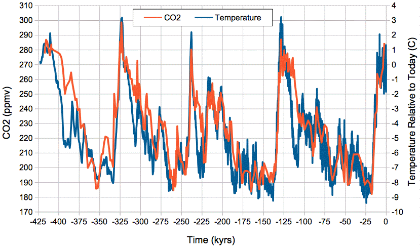
Figure: Absolute Atmospheric CO2 Concentration and Relative Temperature versus Time from Vostok ice cores. Click to enlarge. Local copies of data here and here.
We see close and sustained correlation between CO2 concentration and temperature, even as temperature varies by 12°C. If we assume today's average global temperature is 14°C = 287 K, the change from −9°C to +3°C relative to today is a swing from 278 K to 290 K. Our (Eq. 3) predicts an increase in the mass of carbon in the atmosphere by a factor of e2300(1/278−1/290) = 1.41. Because almost all carbon in the atmosphere is bound up in CO2 molecules, the concentration of CO2 in the atmosphere is proportional to the total mass of carbon in the atmosphere, so when the total mass increases by a factor of 1.41, the CO2 concentration should increase by a factor of 1.41 also. Looking at the graph, we see CO2 rising from 190 ppmv to 290 ppmv, which is a factor of 1.52. Given the many uncertainties in our calculations, and in the ice-core measurements themselves, we are well-satisfied with the agreement between our calculations and the magnitude of the CO2 concentration changes in the ice core measurements.
We conclude that the correlation between CO2 concentration and temperature in the Earth's atmosphere over the past half million years is due to the effect of temperature upon the exchange of CO2 between the atmosphere and the oceanic reservoir of the Earth's carbon cycle. As the temperature rises, the CO2 concentration rises, and when temperature falls, the CO2 concentration falls.
Appendix 1: The van t'Hoff equation for CO2 and water states that the concentration of CO2 above the water is proportional to e−2400/T. Our (Eq. 2) states that it is proportional to e−2300/T. We are well-satisfied with this agreement.
Appendix 2: Suppose we have pure CO2 gas at atmospheric pressure above a reservoir of water. No matter how much CO2 the water dissolves, we maintain the same pressure of CO2 above the water. In this arrangement, unlike the arrangement of our carbon cycle, the concentration of CO2 in the water can vary. Applying the same reasoning we presented in our previous post, the rate at which CO2 molecules are absorbed by the water remains constant with temperature. At equilibrium, the rate at which CO2 molecules are emitted by the water must equal the rate at which they are absorbed, which means the rate of emission must also remain constant. But our calculation states that the probability of any given CO2 molecule in the water being emitted in a certain interval of time must increase with temperature as e−2300/T. If the rate of emission is to remain constant, the concentration of CO2 in the water must decrease with temperature as e2300/T. Only then will the rate of CO2 emission by the water, which is the product of the probability and the concentration, remain constant with temperature. We examine the plot of CO2 solubility in water versus temperature here. As temperature increases from 10°C to 20°C, the solubility of CO2 in water drops from 2.5 g/kg to 1.25 g/kg, which is a factor of 0.50. Our calculation suggests that it should drop by a factor of 0.58. We are well-satisfied with this agreement.
Tuesday, January 5, 2016
Carbon Cycle: Effect of Temperature
Up to now, we assumed that the temperature of our carbon cycle remained constant. We never specified what the temperature of the ocean or the atmosphere was. Nor did we assume that the temperature of the ocean or the atmosphere was uniform. We merely assumed that the temperature in each part of the system remained constant. Today we estimate how the rate of transfer coefficients of our carbon cycle, kA and kR, will change with temperature. We recall that kA is the fraction of atmospheric CO2 molecules that will be absorbed by the oceanic reservoir each year, and kR is the fraction of oceanic reservoir CO2 molecules that will be emitted into the atmosphere each year.
Claim: To the first approximation, kA is independent of temperature.
Justification: Absorption of CO2 takes place at the surface of the ocean. The air pressure at sea-level is dictated by the weight of air per square meter pressing on the sea, which is roughly ten tonnes per square meter. When the atmosphere warms up, its mass does not change. The pressure at sea-level remains constant. But the air does expand. Because the air expands, the number of CO2 molecules per cubic meter decreases. Because the gas is warmer, each CO2 molecule is moving faster. Their average velocity is proportional to the square root of the absolute temperature. Suppose we increase the temperature from 14°C to 15°C. Absolute temperature increases from 287 K to 288 K. According to the gas law, the number of CO2 molecules per cubic meter at the ocean surface decreases by 0.35%. But their velocity increases by 0.18%, which means each CO2 molecule above the ocean surface collides with the ocean 0.18% more frequently than before. Combining these two effects, there will be a net 0.18% decrease in the number of opportunities for CO2 molecules to be absorbed. To the first approximation, this is no change at all. Let us also consider whether a faster-moving CO2 molecule, having collided with the ocean, is more or less likely to be absorbed. When CO2 dissolves in water, energy is released. The CO2 molecule does not need to supply any energy in order to be dissolved. A hotter CO2 molecule has more energy, but this energy is not required by dissolution, and will not make the reaction more likely. To the first approximation, therefore, a 1°C rise in temperature will have no significant effect upon kA.
Claim: To the first approximation, KR increases by a factor of 1.028 for each 1°C warming of the ocean surface.
Justification: Emission of CO2 takes place at the surface of the ocean. When the ocean warms by 1°C, its volume increases by 0.02%, which is insignificant. As we showed above, the warmer CO2 molecules will collide with the ocean surface 0.18% more often, but this, too, is insignificant. Let us consider whether a faster-moving CO2 molecule, having reached the surface of the ocean, is more or less likely to be emitted into the atmosphere. The emission of CO2 from solution requires heat. The enthalpy of dissolution for CO2 in water is −19.4 kJ/mole = −0.20 eV per CO2 molecule. (Compare to 0.42 eV latent heat of vaporization and −0.062 eV latent heat of fusion for an H20 molecule, and 0.26 eV latent heat of sublimation for a CO2 molecule.) Each CO2 molecule dissolving in water releases 0.20 eV of heat. Conversely, in order to be un-dissolved, a CO2 molecule needs to supply at least 0.20 eV from its own thermal energy. At 14°C, the average molecule has kinetic energy only 0.025 eV. But a tiny fraction will have, by random collisions, a much higher energy, as dictated by the Boltzmann distribution. In a given period of time, the number of molecules that attain energy E is proportional to e−E/kT, where T is absolute temperature, k = 8.62×10⁻⁵ eV/K is the Boltzmann constant, and e = 2.72 is the exponential constant. The rate at which any reaction requiring thermal energy E takes place is proportional to e−E/kT. Thus kR is proportional to e−E/kT, which means there is some constant, A, with units of 1/yr, for which kR = A e−0.2/0.0000862T = Ae−2300/T. In our natural, equilibrium carbon cycle, kR = 0.00048 1/yr. Suppose the natural, equilibrium temperature of the ocean surface is 14°C = 287 K. We can obtain the value of A as follows.
kR @ 287K = Ae−2300/287 = A×0.00033 = 0.00048 1/yr ⇒ A = 1.45 1/yr.
We raise the temperature by 1°C to 15°C = 288 K and re-calculate the rate.
kR @ 288K = 1.45 e−2300/288 = 0.000493 1/yr.
The rate has increased by a factor of 0.000493/0.00048 = 1.028, which is 2.8%. If we use 10°C or 20°C as our initial ocean temperature, we get 2.9% and 2.7% rises respectively. To the first approximation, each 1°C increase in temperature increases kR by 2.8%, regardless of our guess at the initial temperature of the ocean surface.
We simulate the effect of a sudden 1°C warming of our carbon cycle in the following way. We begin with our natural, equilibrium atmosphere, described by our carbon cycle model. We increase kR by 2.8%. We set the fossil fuel emission, mF, to zero. We obtain the following plot of atmospheric CO2 concentration versus time.

Figure: Atmospheric CO2 Concentration Following a 1°C Step Increase in Temperature.
The increase in temperature causes an immediate 2.8% increase in the rate at which CO2 is emitted by the ocean, but no increase in the rate at which it is absorbed. The additional CO2 released by the ocean builds up in the atmosphere. As the concentration of CO2 in the atmosphere increases, the rate at which it is absorbed by the ocean increases, because there are more CO2 molecules available for absorption. When the atmospheric concentration has increased by 2.8%, the rate of absorption is once again equal to the rate of emission. The carbon cycle reaches its new equilibrium in roughly one hundred years.
In our next post, we will see how well our calculations agree with the many empirical observations of carbon dioxide in solution, and with the history of our atmosphere over the past half-million years.
Claim: To the first approximation, kA is independent of temperature.
Justification: Absorption of CO2 takes place at the surface of the ocean. The air pressure at sea-level is dictated by the weight of air per square meter pressing on the sea, which is roughly ten tonnes per square meter. When the atmosphere warms up, its mass does not change. The pressure at sea-level remains constant. But the air does expand. Because the air expands, the number of CO2 molecules per cubic meter decreases. Because the gas is warmer, each CO2 molecule is moving faster. Their average velocity is proportional to the square root of the absolute temperature. Suppose we increase the temperature from 14°C to 15°C. Absolute temperature increases from 287 K to 288 K. According to the gas law, the number of CO2 molecules per cubic meter at the ocean surface decreases by 0.35%. But their velocity increases by 0.18%, which means each CO2 molecule above the ocean surface collides with the ocean 0.18% more frequently than before. Combining these two effects, there will be a net 0.18% decrease in the number of opportunities for CO2 molecules to be absorbed. To the first approximation, this is no change at all. Let us also consider whether a faster-moving CO2 molecule, having collided with the ocean, is more or less likely to be absorbed. When CO2 dissolves in water, energy is released. The CO2 molecule does not need to supply any energy in order to be dissolved. A hotter CO2 molecule has more energy, but this energy is not required by dissolution, and will not make the reaction more likely. To the first approximation, therefore, a 1°C rise in temperature will have no significant effect upon kA.
Claim: To the first approximation, KR increases by a factor of 1.028 for each 1°C warming of the ocean surface.
Justification: Emission of CO2 takes place at the surface of the ocean. When the ocean warms by 1°C, its volume increases by 0.02%, which is insignificant. As we showed above, the warmer CO2 molecules will collide with the ocean surface 0.18% more often, but this, too, is insignificant. Let us consider whether a faster-moving CO2 molecule, having reached the surface of the ocean, is more or less likely to be emitted into the atmosphere. The emission of CO2 from solution requires heat. The enthalpy of dissolution for CO2 in water is −19.4 kJ/mole = −0.20 eV per CO2 molecule. (Compare to 0.42 eV latent heat of vaporization and −0.062 eV latent heat of fusion for an H20 molecule, and 0.26 eV latent heat of sublimation for a CO2 molecule.) Each CO2 molecule dissolving in water releases 0.20 eV of heat. Conversely, in order to be un-dissolved, a CO2 molecule needs to supply at least 0.20 eV from its own thermal energy. At 14°C, the average molecule has kinetic energy only 0.025 eV. But a tiny fraction will have, by random collisions, a much higher energy, as dictated by the Boltzmann distribution. In a given period of time, the number of molecules that attain energy E is proportional to e−E/kT, where T is absolute temperature, k = 8.62×10⁻⁵ eV/K is the Boltzmann constant, and e = 2.72 is the exponential constant. The rate at which any reaction requiring thermal energy E takes place is proportional to e−E/kT. Thus kR is proportional to e−E/kT, which means there is some constant, A, with units of 1/yr, for which kR = A e−0.2/0.0000862T = Ae−2300/T. In our natural, equilibrium carbon cycle, kR = 0.00048 1/yr. Suppose the natural, equilibrium temperature of the ocean surface is 14°C = 287 K. We can obtain the value of A as follows.
kR @ 287K = Ae−2300/287 = A×0.00033 = 0.00048 1/yr ⇒ A = 1.45 1/yr.
We raise the temperature by 1°C to 15°C = 288 K and re-calculate the rate.
kR @ 288K = 1.45 e−2300/288 = 0.000493 1/yr.
The rate has increased by a factor of 0.000493/0.00048 = 1.028, which is 2.8%. If we use 10°C or 20°C as our initial ocean temperature, we get 2.9% and 2.7% rises respectively. To the first approximation, each 1°C increase in temperature increases kR by 2.8%, regardless of our guess at the initial temperature of the ocean surface.
We simulate the effect of a sudden 1°C warming of our carbon cycle in the following way. We begin with our natural, equilibrium atmosphere, described by our carbon cycle model. We increase kR by 2.8%. We set the fossil fuel emission, mF, to zero. We obtain the following plot of atmospheric CO2 concentration versus time.
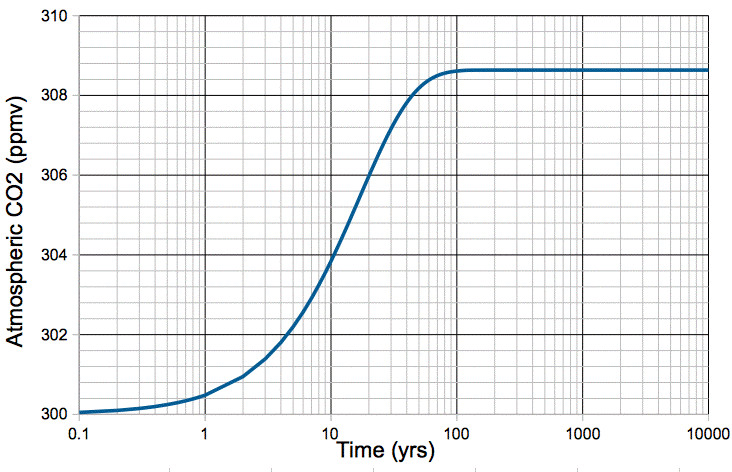
Figure: Atmospheric CO2 Concentration Following a 1°C Step Increase in Temperature.
The increase in temperature causes an immediate 2.8% increase in the rate at which CO2 is emitted by the ocean, but no increase in the rate at which it is absorbed. The additional CO2 released by the ocean builds up in the atmosphere. As the concentration of CO2 in the atmosphere increases, the rate at which it is absorbed by the ocean increases, because there are more CO2 molecules available for absorption. When the atmospheric concentration has increased by 2.8%, the rate of absorption is once again equal to the rate of emission. The carbon cycle reaches its new equilibrium in roughly one hundred years.
In our next post, we will see how well our calculations agree with the many empirical observations of carbon dioxide in solution, and with the history of our atmosphere over the past half-million years.
Wednesday, April 4, 2012
Conclusion
The anthropogenic global warming (AGW) hypothesis presented by the majority of today's climatologists has two parts. First it claims that the world is getting exceptionally warm, and second it claims that human carbon dioxide (CO2) emissions are the cause of this warming. Seven years ago, we began our personal investigation of this hypothesis, and we did so by considering whether or not the world was indeed getting exceptionally warm.
The first thing we did was estimate the uncertainty inherent in the measurements of global surface temperature. We concluded that natural variations in local climate introduce an error of roughly 0.14°C in the measurement of the change in temperature between any two points in time. The fact that the error is constant with the time over which we measure the change is a consequence of the particular characteristics of local climate fluctuations.
We downloaded the weather station data from NCDC and calculated the global surface anomaly using a method we called integrated derivatives, but which others have called first differences. The graph we obtained was almost identical to the one obtained by CRU using their complex reference grid method. It remains a mystery to us why institutions like CRU, NASA, and NCDC use such a complex method when a far simpler one will do. All graphs show roughly a 0.6°C rise in global surface temperature from 1950 to 2000. This rise is significant compared to our expected resolution of 0.14°C.
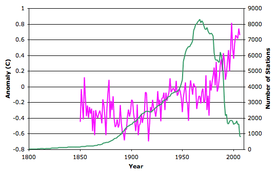
We made this plot superimposing the number of weather stations and the global surface anomaly versus time. The number of weather stations drops dramatically from 1960 and 1990. Only one in four remain active at the end of this thirty-year period. During the same period, the global surface anomaly shows a 0.6°C rise. By selecting subsets of the weather stations, we found that the apparent warming from 1950 to 1990 varied from 0.3°C to 1.0°C depending upon whether we used stations that disappeared in that period, persisted through that period, or existed shorter or longer intervals in the same century. Thus is seemed to us that some significant amount of work would have to be done to eliminate the change in the number of weather stations as a source of error in the data. But we saw no mention whatsoever of this source of error in published papers in which the global surface anomaly is presented, such as Jones et al..
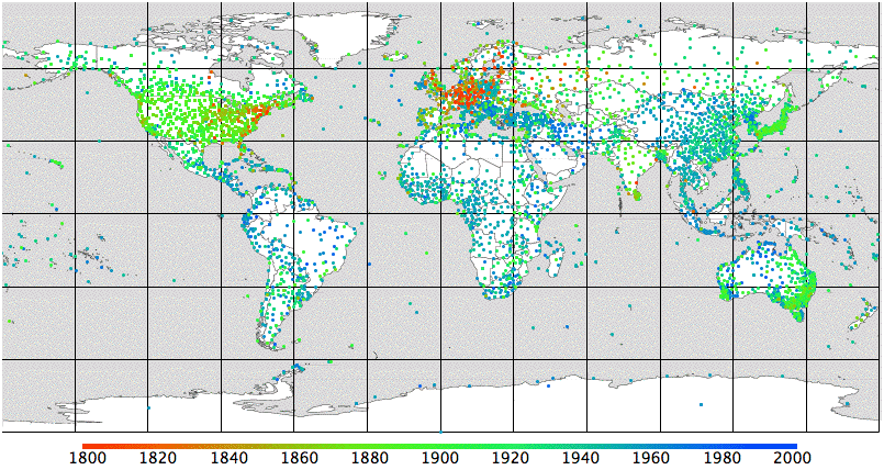
We plotted a global map of the available weather stations, color-coded to show the date they first started reporting. The map shows that almost all stations in the tropics began operating after 1930, while most of those in the temperate regions were operating by 1880. This seems to us to be another source of systematic error in our measurement of the global surface anomaly.
Weather stations might also be affected by the appearance of buildings, tarmac, and road traffic. We found examples of weather stations in which such urban heating caused an apparent warming of several degrees centigrade over a few decades. It seemed to us that this effect would have to be examined in depth by any paper presenting a global surface trend. But papers such as Jones et al. do not address the urban heating issue directly. Instead, they claim that the effect is negligible and refer to other papers as proof. But when we looked up those other papers, we did not find any such proof.
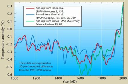
In order to argue that modern temperatures were exceptionally warm, climatologists produced the hockey stick graph, in which a collection of potential long-term measurements of global surface temperature were combined together under the assumption that they could be trusted only to the extent that they showed a temperatures increase from 1950 to 2000. Indeed, if a measurement showed a temperature decline in that period, the hockey stick method would flip the trend over and add it to the combination so that it now contributed to a rise in the same period.
The hockey-stick graph shows no sign of the Medieval Warm Period, in which Greenland was inhabited by farmers, nor the Little Ice Age, when the Thames was known to freeze over, and nor should we expect it to. Given a random set of measurements, the hockey-stick combination method will almost always produce a graph that shows a sharp rise from 1950 to 2000 and a gentle descent during the thousand years before-hand. When applied to the existing measurements of temperature by tree rings, ice cores, and other such indirect methods, it is no surprise that the method produced that same shape.
We presented our doubts about the surface temperature measurements and the hockey stick graph to believers in the AGW hypothesis. We were received with disdain and given no satisfactory answers. Furthermore, the Climategate affair revealed several significant breaches of scientific method by the climate science community. For example, in this graph produced by climatologists for the World Health Organization, the authors removed the tree ring temperature data from 1960 onwards because it showed a decline in temperature, and substituted temperature station measurements in their place. They plotted the combination as a single line. When I asked a prominent climatologists what exactly had been done, he said, "The smooth was calculated using instrumental data past 1960." He declared that a better way to handle the divergence of the tree-ring data from the station measurements would be to cut short the graph of tree-ring data at 1960, so as to hide the decline in temperatures measured by the tree rings.
What we see here is the assumption by climatologists that the world has been warming up and that the global temperature measured by weather stations is correct. This assumption leads them to delete conflicting data on the grounds that it must be bad data. Thus it becomes impossible for them to discover that their assumption is incorrect. By this time, we were skeptical of the global surface anomaly we obtained from the station data. We were no longer certain that the data itself had not been modified by NCDC. We had little reason to trust any other measurement produced by climatologists, we were unimpressed with the hockey-stick method of combining measurements, and we were quite certain that recent temperatures were not exceptional for the past ten thousand years.
We turned our attention to the second part of the AGW hypothesis: the one that says doubling the atmosphere's CO2 concentration will increase the surface temperature by roughly 3°C. It took us a long time to come to a conclusion on this one. The climate models upon which such predictions are based are private property of various climatologists. In any event, we do not trust models produced by a community that is willing to delete data that conflict with its assumptions. If they are willing to delete data, we must assume that they are willing to adjust their models until the models give predictions consistent with their AGW hypothesis.
We began with some laboratory experiments on radiation. We stated the principle of the greenhouse effect. After a great deal of searching around, we eventually obtained the absorption spectrum of various layers of the Earth's atmosphere. This allowed us to confirm that, if the skies remained clear, a doubling of CO2 concentration would cause the world to warm up by about 1.5°C.
But of course the skies don't remain clear. The formation of clouds is a strong function of surface temperature. If the world warms up, there will be more clouds. They will reflect more of the Sun's light, while at the same time, slowing down the radiation of heat into space by the Earth. To determine how these two effects would interact, we built our own climate model, which we called Circulating Cells.
When it comes to determining the effect of increased cloud cover, the most critical parameter to decide upon is the reflection of sunlight by clouds per millimeter of water depth in the cloud. It seemed to us that there should be a large body of literature written recently upon this subject because it is so important to climate modeling. The best paper we found upon the subject was written in 1948, Reflection, Absorption, and Transmission of Insolation by Stratus Cloud. We found a couple of more recent papers about reflection, such as this one, but they do not attempt to provide an empirical formula for the reflection of clouds with increasing cloud depth. We concluded that climatologists are not examining this issue in detail.
In a long sequence of small steps, we built up our climate model until it implemented surface convection, surface heat capacity, evaporation, cloud formation, precipitation, and radiation by clouds. We tested every aspect of the simulation in detail, and based its operating parameters upon our own estimates and upon whatever measurements we could find in climate science journals. We did not choose our model parameters to suit any hypothesis of our own, nor could we have done, because we did not have a model capable of testing the AGW hypothesis until the final stage, and we did not change the parameters in that final stage.
The latest version of our climate model shows that cloud cover increases rapidly as the surface warms above the freezing point of water. The evaporation rate of water from the surface increases approximately as the square of the temperature above freezing, and the only way for water to return to the surface is to form a cloud first. If we ignore the increased reflection of sunlight due to increasing cloud cover, and consider only the slowing-down of radiation into space by the same increase in cloud cover, our model shows roughly 3°C of warming due to a doubling in CO2 concentration. But when we take account of the increased reflection of sunlight by the increasing cloud cover, the warming drops to 0.9°C.
It seems to us that the climate models used by climatologists ignore the reflection of sunlight due to clouds. They may allow for some fixed fraction of sunlight to be reflected by clouds, but they do not allow this fraction to increase with increasing surface temperature. Thus they conclude that the warming due to CO2 doubling will be 3°C. If they took account of the increased reflection, the effect would be far smaller and less dramatic: roughly 1°C.
Doubling the CO2 concentration of the atmosphere will indeed encourage the world to warm up, but not by enough that we should worry. Right now CO2 concentration has increased from roughly 300 ppm to 400 ppm in the past century. If it gets to 600 ppm then we can say that the rise in CO2 concentration will tend to warm the Earth by 1°C. But we are unlikely to be able to check our calculations, because the natural variation in the Earth's climate is itself of order ±1°C from one century to the next.
And so we find ourselves at the end of our journey. Modern warming is not exceptional, and doubling the CO2 concentration will cause the world to warm up by roughly 1°C, not 3°C. The only part of the AGW theory we have not investigated is its assertion that human CO2 emissions are responsible for the increase in atmospheric CO2 concentration over the past century.
My thanks to those of you who took part in the effort, both by private e-mails and in the comments. I would not have continued the effort without your participation. I hope it is clear that my use of "we" instead of "I" is in recognition of the fact that this has been a group effort. I will continue to answer comments on this site, and I will consider any suggestions of further work. To the first approximation, however: we're done.
The first thing we did was estimate the uncertainty inherent in the measurements of global surface temperature. We concluded that natural variations in local climate introduce an error of roughly 0.14°C in the measurement of the change in temperature between any two points in time. The fact that the error is constant with the time over which we measure the change is a consequence of the particular characteristics of local climate fluctuations.
We downloaded the weather station data from NCDC and calculated the global surface anomaly using a method we called integrated derivatives, but which others have called first differences. The graph we obtained was almost identical to the one obtained by CRU using their complex reference grid method. It remains a mystery to us why institutions like CRU, NASA, and NCDC use such a complex method when a far simpler one will do. All graphs show roughly a 0.6°C rise in global surface temperature from 1950 to 2000. This rise is significant compared to our expected resolution of 0.14°C.
We made this plot superimposing the number of weather stations and the global surface anomaly versus time. The number of weather stations drops dramatically from 1960 and 1990. Only one in four remain active at the end of this thirty-year period. During the same period, the global surface anomaly shows a 0.6°C rise. By selecting subsets of the weather stations, we found that the apparent warming from 1950 to 1990 varied from 0.3°C to 1.0°C depending upon whether we used stations that disappeared in that period, persisted through that period, or existed shorter or longer intervals in the same century. Thus is seemed to us that some significant amount of work would have to be done to eliminate the change in the number of weather stations as a source of error in the data. But we saw no mention whatsoever of this source of error in published papers in which the global surface anomaly is presented, such as Jones et al..
We plotted a global map of the available weather stations, color-coded to show the date they first started reporting. The map shows that almost all stations in the tropics began operating after 1930, while most of those in the temperate regions were operating by 1880. This seems to us to be another source of systematic error in our measurement of the global surface anomaly.
Weather stations might also be affected by the appearance of buildings, tarmac, and road traffic. We found examples of weather stations in which such urban heating caused an apparent warming of several degrees centigrade over a few decades. It seemed to us that this effect would have to be examined in depth by any paper presenting a global surface trend. But papers such as Jones et al. do not address the urban heating issue directly. Instead, they claim that the effect is negligible and refer to other papers as proof. But when we looked up those other papers, we did not find any such proof.
In order to argue that modern temperatures were exceptionally warm, climatologists produced the hockey stick graph, in which a collection of potential long-term measurements of global surface temperature were combined together under the assumption that they could be trusted only to the extent that they showed a temperatures increase from 1950 to 2000. Indeed, if a measurement showed a temperature decline in that period, the hockey stick method would flip the trend over and add it to the combination so that it now contributed to a rise in the same period.
The hockey-stick graph shows no sign of the Medieval Warm Period, in which Greenland was inhabited by farmers, nor the Little Ice Age, when the Thames was known to freeze over, and nor should we expect it to. Given a random set of measurements, the hockey-stick combination method will almost always produce a graph that shows a sharp rise from 1950 to 2000 and a gentle descent during the thousand years before-hand. When applied to the existing measurements of temperature by tree rings, ice cores, and other such indirect methods, it is no surprise that the method produced that same shape.
We presented our doubts about the surface temperature measurements and the hockey stick graph to believers in the AGW hypothesis. We were received with disdain and given no satisfactory answers. Furthermore, the Climategate affair revealed several significant breaches of scientific method by the climate science community. For example, in this graph produced by climatologists for the World Health Organization, the authors removed the tree ring temperature data from 1960 onwards because it showed a decline in temperature, and substituted temperature station measurements in their place. They plotted the combination as a single line. When I asked a prominent climatologists what exactly had been done, he said, "The smooth was calculated using instrumental data past 1960." He declared that a better way to handle the divergence of the tree-ring data from the station measurements would be to cut short the graph of tree-ring data at 1960, so as to hide the decline in temperatures measured by the tree rings.
What we see here is the assumption by climatologists that the world has been warming up and that the global temperature measured by weather stations is correct. This assumption leads them to delete conflicting data on the grounds that it must be bad data. Thus it becomes impossible for them to discover that their assumption is incorrect. By this time, we were skeptical of the global surface anomaly we obtained from the station data. We were no longer certain that the data itself had not been modified by NCDC. We had little reason to trust any other measurement produced by climatologists, we were unimpressed with the hockey-stick method of combining measurements, and we were quite certain that recent temperatures were not exceptional for the past ten thousand years.
We turned our attention to the second part of the AGW hypothesis: the one that says doubling the atmosphere's CO2 concentration will increase the surface temperature by roughly 3°C. It took us a long time to come to a conclusion on this one. The climate models upon which such predictions are based are private property of various climatologists. In any event, we do not trust models produced by a community that is willing to delete data that conflict with its assumptions. If they are willing to delete data, we must assume that they are willing to adjust their models until the models give predictions consistent with their AGW hypothesis.
We began with some laboratory experiments on radiation. We stated the principle of the greenhouse effect. After a great deal of searching around, we eventually obtained the absorption spectrum of various layers of the Earth's atmosphere. This allowed us to confirm that, if the skies remained clear, a doubling of CO2 concentration would cause the world to warm up by about 1.5°C.
But of course the skies don't remain clear. The formation of clouds is a strong function of surface temperature. If the world warms up, there will be more clouds. They will reflect more of the Sun's light, while at the same time, slowing down the radiation of heat into space by the Earth. To determine how these two effects would interact, we built our own climate model, which we called Circulating Cells.
When it comes to determining the effect of increased cloud cover, the most critical parameter to decide upon is the reflection of sunlight by clouds per millimeter of water depth in the cloud. It seemed to us that there should be a large body of literature written recently upon this subject because it is so important to climate modeling. The best paper we found upon the subject was written in 1948, Reflection, Absorption, and Transmission of Insolation by Stratus Cloud. We found a couple of more recent papers about reflection, such as this one, but they do not attempt to provide an empirical formula for the reflection of clouds with increasing cloud depth. We concluded that climatologists are not examining this issue in detail.
In a long sequence of small steps, we built up our climate model until it implemented surface convection, surface heat capacity, evaporation, cloud formation, precipitation, and radiation by clouds. We tested every aspect of the simulation in detail, and based its operating parameters upon our own estimates and upon whatever measurements we could find in climate science journals. We did not choose our model parameters to suit any hypothesis of our own, nor could we have done, because we did not have a model capable of testing the AGW hypothesis until the final stage, and we did not change the parameters in that final stage.
The latest version of our climate model shows that cloud cover increases rapidly as the surface warms above the freezing point of water. The evaporation rate of water from the surface increases approximately as the square of the temperature above freezing, and the only way for water to return to the surface is to form a cloud first. If we ignore the increased reflection of sunlight due to increasing cloud cover, and consider only the slowing-down of radiation into space by the same increase in cloud cover, our model shows roughly 3°C of warming due to a doubling in CO2 concentration. But when we take account of the increased reflection of sunlight by the increasing cloud cover, the warming drops to 0.9°C.
It seems to us that the climate models used by climatologists ignore the reflection of sunlight due to clouds. They may allow for some fixed fraction of sunlight to be reflected by clouds, but they do not allow this fraction to increase with increasing surface temperature. Thus they conclude that the warming due to CO2 doubling will be 3°C. If they took account of the increased reflection, the effect would be far smaller and less dramatic: roughly 1°C.
Doubling the CO2 concentration of the atmosphere will indeed encourage the world to warm up, but not by enough that we should worry. Right now CO2 concentration has increased from roughly 300 ppm to 400 ppm in the past century. If it gets to 600 ppm then we can say that the rise in CO2 concentration will tend to warm the Earth by 1°C. But we are unlikely to be able to check our calculations, because the natural variation in the Earth's climate is itself of order ±1°C from one century to the next.
And so we find ourselves at the end of our journey. Modern warming is not exceptional, and doubling the CO2 concentration will cause the world to warm up by roughly 1°C, not 3°C. The only part of the AGW theory we have not investigated is its assertion that human CO2 emissions are responsible for the increase in atmospheric CO2 concentration over the past century.
My thanks to those of you who took part in the effort, both by private e-mails and in the comments. I would not have continued the effort without your participation. I hope it is clear that my use of "we" instead of "I" is in recognition of the fact that this has been a group effort. I will continue to answer comments on this site, and I will consider any suggestions of further work. To the first approximation, however: we're done.
Thursday, March 15, 2012
Anthropogenic Global Warming
The Anthropogenic Global Warming (AGW) hypothesis states that doubling the CO2 concentration of the Earth's atmosphere will raise the average surface temperature of the Earth by a minimum of 1.5°C, and more likely 3°C.
In our investigation of the absorption and emission of long-wave radiation by the Earth's atmosphere, we calculated that a sudden doubling of CO2 concentration would decrease the power the Earth radiates into space by 6.6 W/m2. We then estimated how much the Earth and its atmosphere would have to warm up in order to restore the heat radiated into space to its original value. We assumed there would be no significant change in cloud cover as a result of the warming, and we applied Stefan's Law to calculate how the heat radiated by the Earth and its atmosphere would increase. We found that the required increase in surface temperature would be around 1.6°C. If there were no change in cloud cover, then the heat arriving from the Sun would remain the same, and we could expect the Earth to warm up by 1.6°C so as to once again arrive at thermal equilibrium.
The AGW hypothesis states that in the event of the Earth warming, changes in cloud cover will be such as to amplify the warming we calculate using Stefan's Law. Here is an extract from today's entry on Global Warming at Wikipedia.
The main positive feedback in the climate system is the water vapor feedback. The main negative feedback is radiative cooling through the Stefan–Boltzmann law, which increases as the fourth power of temperature.
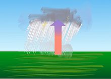
As the Earth warms up, water evaporates more quickly from the oceans. Almost all water that evaporates must turn into clouds before it returns to Earth. Water condensing directly onto grass in the morning is an exception to this rule, but the vast majority of water vapor will return only as rain or snow, and so must first take the form of a cloud.
Clouds absorb long-wave radiation emitted by the Earth's surface, so the Earth cannot radiate its heat directly into space. Instead, the clouds radiate into space and warm the Earth with back radiation. Thus increasing cloud cover means less heat radiated into space for the same surface temperature. This is the positive feedback referred to by the AGW hypothesis. The AGW climate models predict that this positive feedback will amplify the minimum 1.5°C warming caused by CO2 to roughly 3°C. Some say 2°C and other say 4°C, but all agree that the actual warming will be greater than 1.5°C.
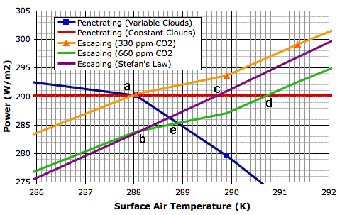
We see this positive feedback in our Circulating Cells simulation, version CC11, which simulates the formation of clouds as well as their absorption and emission of long-wave radiation. The graph below shows a close-up of the behavior of the simulation in the neighborhood of its equilibrium point for 350 W/m2 solar power.

The blue line shows how the power that penetrates to the surface of our simulated planet varies with increasing surface temperature. The orange line shows how the total power escaping from our simulated planet increases with surface temperature. These two lines cross at a, where temperature is 288 K and total escaping power is 290 W/m2. Our simulated atmosphere absorbs 50% of long-wave radiation, which is an adequate approximation of our atmosphere with its current concentration of CO2 (roughly 330 ppm).
The green line is the same as the orange line, but displaced down by 6.6 W/m2, which is the amount by which we calculated the total power escaping from the Earth will decrease if we double CO2 concentration (to roughly 660 ppm). Thus the green line tells us the total escaping power at the same temperature if we were to double the CO2 concentration. Point b on the green line is 288 K, and the total escaping power is 283.4 W/m2.
The purple line shows how the total escaping power will increase from b if we assume the cloud cover is constant and use only Stefan's Law to determine the heat radiated into space by the surface and atmosphere. The red line shows the solar power penetrating to the surface if we assume the cloud cover is constant. With constant cloud cover, the penetrating solar power does not change.
The purple and red lines meet at c, which is 289.6 K, or 1.6°C above the previous equilibrium point. Thus our simulation shows us that the warming due to CO2 doubling, if we ignore changes in cloud cover, will be 1.6°C, which is consistent with our previous calculation.
The green line, however, is the simulation's calculation of the total escaping power for increasing surface temperature. We see that the heat radiated into space does not increase as quickly as Stefan's Law would lead us to expect. And the reason for that is precisely the reason quoted by the AGW hypothesis: increasing cloud cover is slowing down the radiation of heat into space. The green line and the red line intersect at d, which is 290.7 K, or 2.7°C above our original equilibrium temperature. This is the new equilibrium temperature of the planet surface if we double CO2 concentration and we assume that there will be no change in the solar power penetrating to the surface while the cloud cover increases.
But the solar power penetrating to the surface must decrease as cloud cover increases. Clouds reflect sunlight. Thick clouds reflect 90% of solar power back into space. Even thin, high clouds reflect 10%. Increasing cloud cover will decrease the solar power penetrating to the surface. That is why our blue line slopes downwards. This is negative feedback, which acts against the positive feedback described by the AGW theory. The blue line shows how the solar power penetrating to the surface decreases as our cloud cover increases.
The blue line and the green line intersect at e, which is the equilibrium point we arrive at after doubling the CO2 concentration and considering both the positive feedback of back-radiation and the negative feedback of solar reflection. The temperature at e is 288.9 K, which is 0.9°C above our original equilibrium temperature.
Thus our simulation shows how the negative feedback generated by clouds dominates their positive feedback, and suggests that the actual warming of the Earth's surface due to a doubling of CO2 will be closer to 0.9°C than the 3°C predicted by the AGW hypothesis.
In our investigation of the absorption and emission of long-wave radiation by the Earth's atmosphere, we calculated that a sudden doubling of CO2 concentration would decrease the power the Earth radiates into space by 6.6 W/m2. We then estimated how much the Earth and its atmosphere would have to warm up in order to restore the heat radiated into space to its original value. We assumed there would be no significant change in cloud cover as a result of the warming, and we applied Stefan's Law to calculate how the heat radiated by the Earth and its atmosphere would increase. We found that the required increase in surface temperature would be around 1.6°C. If there were no change in cloud cover, then the heat arriving from the Sun would remain the same, and we could expect the Earth to warm up by 1.6°C so as to once again arrive at thermal equilibrium.
The AGW hypothesis states that in the event of the Earth warming, changes in cloud cover will be such as to amplify the warming we calculate using Stefan's Law. Here is an extract from today's entry on Global Warming at Wikipedia.
The main positive feedback in the climate system is the water vapor feedback. The main negative feedback is radiative cooling through the Stefan–Boltzmann law, which increases as the fourth power of temperature.
As the Earth warms up, water evaporates more quickly from the oceans. Almost all water that evaporates must turn into clouds before it returns to Earth. Water condensing directly onto grass in the morning is an exception to this rule, but the vast majority of water vapor will return only as rain or snow, and so must first take the form of a cloud.
Clouds absorb long-wave radiation emitted by the Earth's surface, so the Earth cannot radiate its heat directly into space. Instead, the clouds radiate into space and warm the Earth with back radiation. Thus increasing cloud cover means less heat radiated into space for the same surface temperature. This is the positive feedback referred to by the AGW hypothesis. The AGW climate models predict that this positive feedback will amplify the minimum 1.5°C warming caused by CO2 to roughly 3°C. Some say 2°C and other say 4°C, but all agree that the actual warming will be greater than 1.5°C.
We see this positive feedback in our Circulating Cells simulation, version CC11, which simulates the formation of clouds as well as their absorption and emission of long-wave radiation. The graph below shows a close-up of the behavior of the simulation in the neighborhood of its equilibrium point for 350 W/m2 solar power.
The blue line shows how the power that penetrates to the surface of our simulated planet varies with increasing surface temperature. The orange line shows how the total power escaping from our simulated planet increases with surface temperature. These two lines cross at a, where temperature is 288 K and total escaping power is 290 W/m2. Our simulated atmosphere absorbs 50% of long-wave radiation, which is an adequate approximation of our atmosphere with its current concentration of CO2 (roughly 330 ppm).
The green line is the same as the orange line, but displaced down by 6.6 W/m2, which is the amount by which we calculated the total power escaping from the Earth will decrease if we double CO2 concentration (to roughly 660 ppm). Thus the green line tells us the total escaping power at the same temperature if we were to double the CO2 concentration. Point b on the green line is 288 K, and the total escaping power is 283.4 W/m2.
The purple line shows how the total escaping power will increase from b if we assume the cloud cover is constant and use only Stefan's Law to determine the heat radiated into space by the surface and atmosphere. The red line shows the solar power penetrating to the surface if we assume the cloud cover is constant. With constant cloud cover, the penetrating solar power does not change.
The purple and red lines meet at c, which is 289.6 K, or 1.6°C above the previous equilibrium point. Thus our simulation shows us that the warming due to CO2 doubling, if we ignore changes in cloud cover, will be 1.6°C, which is consistent with our previous calculation.
The green line, however, is the simulation's calculation of the total escaping power for increasing surface temperature. We see that the heat radiated into space does not increase as quickly as Stefan's Law would lead us to expect. And the reason for that is precisely the reason quoted by the AGW hypothesis: increasing cloud cover is slowing down the radiation of heat into space. The green line and the red line intersect at d, which is 290.7 K, or 2.7°C above our original equilibrium temperature. This is the new equilibrium temperature of the planet surface if we double CO2 concentration and we assume that there will be no change in the solar power penetrating to the surface while the cloud cover increases.
But the solar power penetrating to the surface must decrease as cloud cover increases. Clouds reflect sunlight. Thick clouds reflect 90% of solar power back into space. Even thin, high clouds reflect 10%. Increasing cloud cover will decrease the solar power penetrating to the surface. That is why our blue line slopes downwards. This is negative feedback, which acts against the positive feedback described by the AGW theory. The blue line shows how the solar power penetrating to the surface decreases as our cloud cover increases.
The blue line and the green line intersect at e, which is the equilibrium point we arrive at after doubling the CO2 concentration and considering both the positive feedback of back-radiation and the negative feedback of solar reflection. The temperature at e is 288.9 K, which is 0.9°C above our original equilibrium temperature.
Thus our simulation shows how the negative feedback generated by clouds dominates their positive feedback, and suggests that the actual warming of the Earth's surface due to a doubling of CO2 will be closer to 0.9°C than the 3°C predicted by the AGW hypothesis.
Wednesday, March 7, 2012
Equilibrium Point
Heat arrives at the Earth in the from of sunlight. The clouds reflect some of it. Almost all the rest arrives at the Earth's surface. Of the sunlight that reaches the surface, some is reflected back into space, especially by snow, but most is absorbed. To the first approximation, therefore, sunlight affects the climate only by it warming the surface, not by warming the atmosphere directly.
In our Circulating Cells simulation, version CC11, solar power is either reflected by clouds or absorbed by the surface. The only way for heat to enter the atmosphere is by contact with the surface, so it is the temperature of the surface that drives the the circulation of gases and the creation of clouds, snow, and rain. When we observe, for example, that 80% of solar power is penetrating to the surface when the surface gas temperature is 290 K, we can assume that the 80% of solar power will penetrate to the surface whenever the surface gas temperature is 290 K.
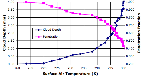
Our program of solar increase provides us with observations of cloud depth and penetrating power for a range of solar powers, and therefore for a range of surface temperatures. The following graph shows how the fraction of solar power penetrating to the surface varies with surface temperature.

In our simulation we calculate the penetrating power for each surface block using the depth of the clouds in the column of cells above the surface block. We cannot, however, use the average cloud depth to obtain a measurement of average penetration fraction. When we do so, our measurement is always too low, because there are gaps in the cloud cover, and these gaps allow more light to pass through than if the clouds were distributed uniformly.
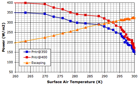
In the following graph, we have taken our measurements of penetration fraction and used them to calculate the power that would penetrate to the surface for two values of solar power: 350 W/m2 and 400 W/m2. Along with these penetrating powers, we also plot the total escaping power.

At thermal equilibrium, the total escaping power must be equal to the penetrating power. Thus the intersection of the penetrating power and escaping power graphs occurs at the equilibrium temperature. For solar power 350 W/m2, the intersection occurs at 288 K. For 400 W/m2, the intersection occurs at 292 K. These are, of course, the same equilibrium temperatures we obtain from our existing graph of surface temperature versus solar power.
In our next post, we will use the above graph and the calculations we presented in With 660 PPM CO2 to estimate how much the Earth would warm up if we doubled the CO2 concentration of its atmosphere.
In our Circulating Cells simulation, version CC11, solar power is either reflected by clouds or absorbed by the surface. The only way for heat to enter the atmosphere is by contact with the surface, so it is the temperature of the surface that drives the the circulation of gases and the creation of clouds, snow, and rain. When we observe, for example, that 80% of solar power is penetrating to the surface when the surface gas temperature is 290 K, we can assume that the 80% of solar power will penetrate to the surface whenever the surface gas temperature is 290 K.
Our program of solar increase provides us with observations of cloud depth and penetrating power for a range of solar powers, and therefore for a range of surface temperatures. The following graph shows how the fraction of solar power penetrating to the surface varies with surface temperature.
In our simulation we calculate the penetrating power for each surface block using the depth of the clouds in the column of cells above the surface block. We cannot, however, use the average cloud depth to obtain a measurement of average penetration fraction. When we do so, our measurement is always too low, because there are gaps in the cloud cover, and these gaps allow more light to pass through than if the clouds were distributed uniformly.
In the following graph, we have taken our measurements of penetration fraction and used them to calculate the power that would penetrate to the surface for two values of solar power: 350 W/m2 and 400 W/m2. Along with these penetrating powers, we also plot the total escaping power.
At thermal equilibrium, the total escaping power must be equal to the penetrating power. Thus the intersection of the penetrating power and escaping power graphs occurs at the equilibrium temperature. For solar power 350 W/m2, the intersection occurs at 288 K. For 400 W/m2, the intersection occurs at 292 K. These are, of course, the same equilibrium temperatures we obtain from our existing graph of surface temperature versus solar power.
In our next post, we will use the above graph and the calculations we presented in With 660 PPM CO2 to estimate how much the Earth would warm up if we doubled the CO2 concentration of its atmosphere.
Friday, March 2, 2012
Conservation of Heat
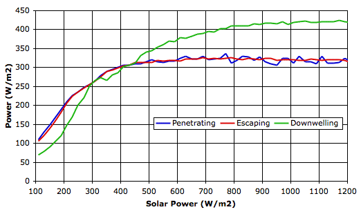
In Solar Increase we were concerned that our program of increasing solar power did not allow adequate time at each value of solar power for the simulation to arrive at thermal equilibrium. As we described in our previous post, we now have measurements of the state of the simulation at each value of solar power. The following graph plots penetrating power, total escaping power, and downwelling power versus solar power. The penetrating power is the power per square meter that gets to the surface through the clouds. The total escaping power is the power per square meter that the surface and atmosphere together radiate into space. The downwelling power is the power arriving back at the surface from the radiating clouds.

The downwelling power is increasing because the cloud layer is getting thicker. The clouds radiating heat towards the surface are lower down and therefore warmer. But it is the equality of the penetrating and escaping power that interests us the most today. At thermal equilibrium, the total escaping power should be equal to the penetrating power. And indeed we see that this appears to be the case for all values of solar power.
The downwelling power is increasing because the cloud layer is getting thicker. The clouds radiating heat towards the surface are lower down and therefore warmer. But it is the equality of the penetrating and escaping power that interests us the most today. At thermal equilibrium, the total escaping power should be equal to the penetrating power. And indeed we see that this appears to be the case for all values of solar power.
Sunday, February 26, 2012
Thickening Clouds
As we describe in Solar Increase, we warmed up our simulated planet by increasing the incoming solar power by 10 W/m2 every two thousand hours of simulated time. Starting from an initial value of 100 W/m2, we increased the solar power to 1200 W/m2 over the course of three weeks of our own time, which corresponds to the passage of over a million hours of simulated time. During the course of the simulation, we recorded the state of the atmospheric array every twenty hours, and these recordings constitute our measurements of the simulated atmosphere during the course of our simulated experiment.
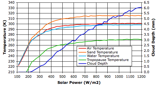
In our pervious post we observed that some properties of the atmosphere, such as penetrating power, fluctuated greatly from one measurement to the next. In order to reduce the influence of these fluctuations, we took the average of the last 500 hours of measurements at each value of incoming solar power, and so obtained a value for each property at each solar power. The graph below shows how some of these properties vary with solar power.

Surface temperature increases hardly at all from 800 W/m2 to 1200 W/m2, and yet cloud cover increases steadily. How can it be that cloud cover increases when the surface temperature, which drives evaporation, hardly increases at all?
In our simulated evaporation cycle, precipitation beings with the formation of snow in air below temperature Tf_droplets. We have this parameter set to 268 K, which is five degrees below the freezing point of water. When solar power reaches 800 W/m2, the average temperature of the tropopause has reached 268 K. Snow can form only in the colder clouds of the tropopause, and nowhere below the tropopause. Each time we increase the solar power, the surface temperature at first warms a little, but within a few hundred hours, this warming reaches the tropopause, where it further slows snow formation, and increases the cloud depth. With more sunlight being reflected back into space, the surface cools again until it is hardly warmer than it started. For solar powers greater than 800 W/m2, an increase of 100 W/m2 causes a substantial increase in cloud depth (roughly 0.5 mm), a slight increase in tropopause temperature (roughly 1 K), and an increase in surface temperature too small for us to detect (less than 0.3 K).
This profound suppression of warming by our simulation is not, however, a good representation of what would happen in the Earth's atmosphere. In our simulation, gas cells that contain clouds cannot rise above our top row of cells, so there is a limit to how much they can cool down. In the Earth's atmosphere, clouds can rise as far as they need to in order to cool down and produce snow rapidly. Thus our simulation is no longer realistic once its tropopause approaches the melting point of ice. We will therefore concentrate our attention upon the behavior of the simulation for solar powers less than 600 W/m2, for which our simulated tropopause is well below the temperature required for the rapid formation of snow.
In our pervious post we observed that some properties of the atmosphere, such as penetrating power, fluctuated greatly from one measurement to the next. In order to reduce the influence of these fluctuations, we took the average of the last 500 hours of measurements at each value of incoming solar power, and so obtained a value for each property at each solar power. The graph below shows how some of these properties vary with solar power.
Surface temperature increases hardly at all from 800 W/m2 to 1200 W/m2, and yet cloud cover increases steadily. How can it be that cloud cover increases when the surface temperature, which drives evaporation, hardly increases at all?
In our simulated evaporation cycle, precipitation beings with the formation of snow in air below temperature Tf_droplets. We have this parameter set to 268 K, which is five degrees below the freezing point of water. When solar power reaches 800 W/m2, the average temperature of the tropopause has reached 268 K. Snow can form only in the colder clouds of the tropopause, and nowhere below the tropopause. Each time we increase the solar power, the surface temperature at first warms a little, but within a few hundred hours, this warming reaches the tropopause, where it further slows snow formation, and increases the cloud depth. With more sunlight being reflected back into space, the surface cools again until it is hardly warmer than it started. For solar powers greater than 800 W/m2, an increase of 100 W/m2 causes a substantial increase in cloud depth (roughly 0.5 mm), a slight increase in tropopause temperature (roughly 1 K), and an increase in surface temperature too small for us to detect (less than 0.3 K).
This profound suppression of warming by our simulation is not, however, a good representation of what would happen in the Earth's atmosphere. In our simulation, gas cells that contain clouds cannot rise above our top row of cells, so there is a limit to how much they can cool down. In the Earth's atmosphere, clouds can rise as far as they need to in order to cool down and produce snow rapidly. Thus our simulation is no longer realistic once its tropopause approaches the melting point of ice. We will therefore concentrate our attention upon the behavior of the simulation for solar powers less than 600 W/m2, for which our simulated tropopause is well below the temperature required for the rapid formation of snow.
Thursday, February 23, 2012
Solar Increase Continued
Today we continue our previous post without any preamble. The graph below shows how our simulated atmosphere warms up as we increase the solar power from one hundred to twelve hundred Watts per square meter. The green line shows how we increased the solar power over the course of twelve simulated years. The blue line shows how the power penetrating to the surface varied with time. The red line is the average temperature of the air resting upon the surface of our simulated planet.

At first, when the sky is clear, the solar power and the penetrating power are equal. But when the solar power reaches 300 W/m2 clouds form and the penetrating power drops below the solar power. As solar power increases from 600 W/m2 to 1200 W/m2, fluctuations in the penetrating power double in their extent, but the average penetrating power appears to remain unchanged. The negative feedback generated by the evaporation cycle is so powerful that the surface air temperature increases by only a few degrees while we double the solar power.
The following screen shot shows the state of the simulation after two thousand hours at 1210 W/m2. You can download this state as a text file SIC_1210W and load it into CC11 to watch the vigorous formation of clouds and descent of precipitation.

We now have the data we need to plot graphs of surface temperature and other properties of the simulation versus solar power.
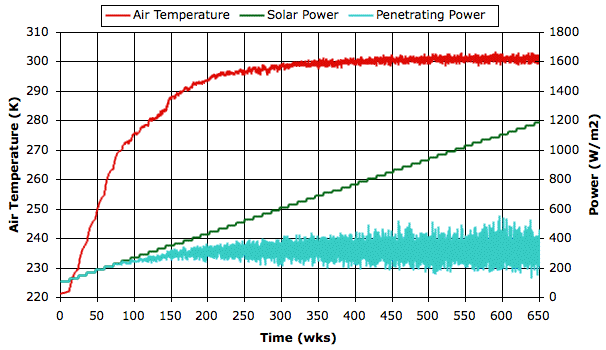
At first, when the sky is clear, the solar power and the penetrating power are equal. But when the solar power reaches 300 W/m2 clouds form and the penetrating power drops below the solar power. As solar power increases from 600 W/m2 to 1200 W/m2, fluctuations in the penetrating power double in their extent, but the average penetrating power appears to remain unchanged. The negative feedback generated by the evaporation cycle is so powerful that the surface air temperature increases by only a few degrees while we double the solar power.
The following screen shot shows the state of the simulation after two thousand hours at 1210 W/m2. You can download this state as a text file SIC_1210W and load it into CC11 to watch the vigorous formation of clouds and descent of precipitation.
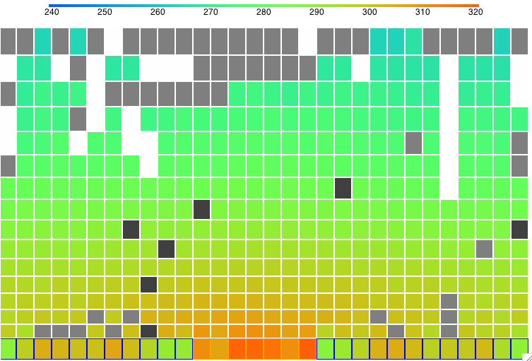
We now have the data we need to plot graphs of surface temperature and other properties of the simulation versus solar power.
Monday, February 13, 2012
Solar Increase
In our previous post we cooled down our simulated atmosphere by reducing the incoming solar power to 100 W/m2. We gave the simulation plenty of time to reach equilibrium, and it arrived at the state RC_100W. The sky is clear. All the Sun's power penetrates to the surface. The surface temperature is −50°C.
We started CC11 from this equilibrium state. We increased the solar power to 110 W/m2. After two thousand hours of simulated time, we increased the solar power to 130 W/m2. We ran for another two thousand hours of simulated time, after which we increased the solar power again. The program performs the solar Increases automatically, so we were able to walk away from the computer and let the simulation run on its own.
The following graph shows surface temperature and solar power plotted against simulation time in weeks. The purpose of this plot is to determine if our simulation reaches equilibrium at each value of solar power.

Below 270 K, we see see the surface temperature is still increasing two thousand hours after the increases in solar power. Perhaps ten thousand hours at each step would be enough. But we are faced with a practical problem of execution time: it took one full week for us to obtain the graph above, with a computer dedicated to the job running continuously.
Once the surface temperature gets above 270 K, however, the evaporation cycle starts up and we see the effects of negative feedback. The changes that result from increases in solar power are markedly smaller and they establish themselves more quickly. Thus our program of solar Increase appears to be gradual enough for temperatures above 270 K, and these are the temperatures we are most interested in.
The following figure shows the equilibrium state of the atmosphere with 490 W/m2 solar power. The running simulation shows vigorous cloud formation and precipitation. You can view this for yourself by downloading CC11, loading state SI_490 into the program, setting Q_sun to 490 in the configuration panel, and pressing Run.

By next week, we hope to have obtained the equilibrium state of our simulation for solar powers 100 W/m2 all the way up to 900 W/m2.
We started CC11 from this equilibrium state. We increased the solar power to 110 W/m2. After two thousand hours of simulated time, we increased the solar power to 130 W/m2. We ran for another two thousand hours of simulated time, after which we increased the solar power again. The program performs the solar Increases automatically, so we were able to walk away from the computer and let the simulation run on its own.
The following graph shows surface temperature and solar power plotted against simulation time in weeks. The purpose of this plot is to determine if our simulation reaches equilibrium at each value of solar power.
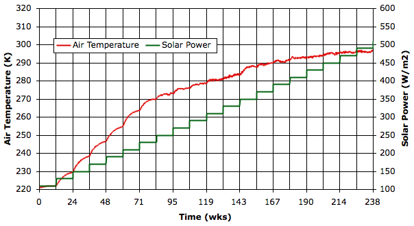
Below 270 K, we see see the surface temperature is still increasing two thousand hours after the increases in solar power. Perhaps ten thousand hours at each step would be enough. But we are faced with a practical problem of execution time: it took one full week for us to obtain the graph above, with a computer dedicated to the job running continuously.
Once the surface temperature gets above 270 K, however, the evaporation cycle starts up and we see the effects of negative feedback. The changes that result from increases in solar power are markedly smaller and they establish themselves more quickly. Thus our program of solar Increase appears to be gradual enough for temperatures above 270 K, and these are the temperatures we are most interested in.
The following figure shows the equilibrium state of the atmosphere with 490 W/m2 solar power. The running simulation shows vigorous cloud formation and precipitation. You can view this for yourself by downloading CC11, loading state SI_490 into the program, setting Q_sun to 490 in the configuration panel, and pressing Run.
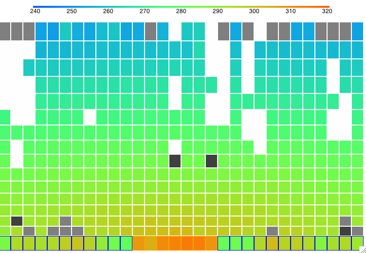
By next week, we hope to have obtained the equilibrium state of our simulation for solar powers 100 W/m2 all the way up to 900 W/m2.
Monday, February 6, 2012
A Big Chill
In Negative Feeback, we increased our simulation's incoming solar power from 200 W/m2 to 400 W/m2 and saw the surface warm by only a 5°C. It turned out that the increasing solar power was almost entirely compensated for by an increase in cloud thickness, so that the power penetrating to the surface remained almost constant. We now ask ourselves, what will happen if we drop the solar power all the way down to 100 W/m2? Will our Radiating Clouds be able to stop the world from cooling?
We started our Circulating Cells program (CC11) in its equilibrium state for 350 W/m2 solar power (RC_14000hr), and reduced the solar power to 100 W/m2. The following graph shows surface air temperature and atmospheric cloud depth for the first five hundred hours.

In the first ten hours, the surface temperature drops by a few degrees. This is what we might expect during one of Earth's nights. After three hundred hours, the surface temperature has dropped to −5°C and there are hardly any clouds left in the sky. The following graph shows the world cooling down to a new, clear-sky equilibrium of −50°C. The graph also shows the solar power penetrating to the surface. Once the sky clears, the penetration is exactly equal to 100 W/m2. We saved the final state of the atmosphere in RC_100W.

We conclude that 100 W/m2 is insufficient solar power to warm the Earth above the freezing point of water, and therefore insufficient solar power to generate the cycle of evaporation and precipitation that stabilizes our climate.
We started our Circulating Cells program (CC11) in its equilibrium state for 350 W/m2 solar power (RC_14000hr), and reduced the solar power to 100 W/m2. The following graph shows surface air temperature and atmospheric cloud depth for the first five hundred hours.
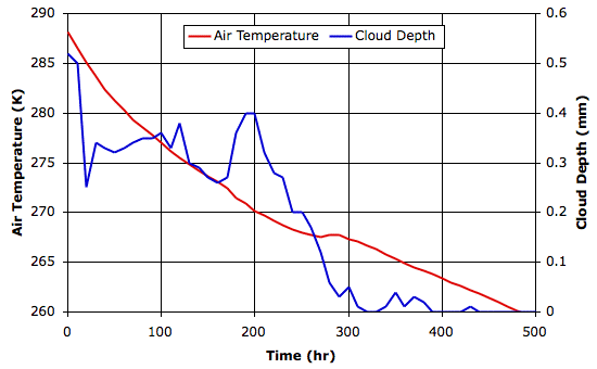
In the first ten hours, the surface temperature drops by a few degrees. This is what we might expect during one of Earth's nights. After three hundred hours, the surface temperature has dropped to −5°C and there are hardly any clouds left in the sky. The following graph shows the world cooling down to a new, clear-sky equilibrium of −50°C. The graph also shows the solar power penetrating to the surface. Once the sky clears, the penetration is exactly equal to 100 W/m2. We saved the final state of the atmosphere in RC_100W.
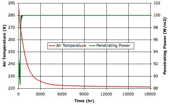
We conclude that 100 W/m2 is insufficient solar power to warm the Earth above the freezing point of water, and therefore insufficient solar power to generate the cycle of evaporation and precipitation that stabilizes our climate.
Monday, January 30, 2012
Lapse Rate
Our Radiating Clouds simulation uses 350 W/m2 for incoming solar power. We know from our Solar Heat calculation that this is the average power arriving at the Earth from the Sun. Our hope is that the lapse rate and surface temperature of our simulation will agree well with the actual lapse rate and surface temperature of the Earth's atmosphere. In the design of our simulation, however, we have made no effort to adjust its parameters to bring about such an agreement.
In the figure below, the blue graph shows temperature versus altitude for thermal equilibrium in the wet atmosphere of our Radiating Clouds simulation. We loaded the equilibrium state, RC_14000hr, into CC11 and instructed the simulation to print temperatures and altitudes.

For comparison, we went back to Simulated Planet Surface and loaded the equilibrium state, Day_4, which arises with the same solar heat, but with the surface entirely made of sand. Thus the pink graph shows temperature versus altitude in a dry atmosphere.
The equilibrium state of the dry atmosphere, which looks like this, shows a linear drop in temperature with altitude. According to our calculations, this slope should be −g/Cp, where g is gravity and Cp is the specific heat capacity of the dry gas. Our simulation uses 10 N/kg for gravity and 1003 J/K for Cp, so the slope of the pink graph should be close to −0.010 K/m. Its actual slope is −0.011 K/m.
The equilibrium state of the wet atmosphere, which looks like this, shows a linear drop in temperature only between altitudes 2 km and 4 km. Near the surface of the planet, the heat liberated by condensing water vapor into rising air reduces the amount by which air cools as it rises. In the tropopause, radiation from the planet surface is absorbed by the tropopause clouds, causing them to be warmer than the air immediately below. In the linear region of the graph, the slope is −0.011 K/m, but if we simply divide the total drop in temperature by the altitude of the tropopause, we obtain a net slope of −0.008 K/m.
Looking at graphs such as these, it appears that the Earth's atmosphere has a lapse rate of around −0.0065 K/m. Our simulation does not come up with this lapse rate exactly, but we see that the introduction of water does cause a substantial reduction in the net lapse rate, and with this we are well-satisfied.
The average temperature of the surface of the Earth is around 14°C, or 287 K. This is the average temperature of the air just above the planet surface, not the temperature of the surface itself. The thermometers we use to measure the surface temperature are several meters above the ground. When we use dry air and a sandy surface in our simulation, the average temperature of the surface air is 298 K. But when we add radiating clouds, rain, and snow, the average temperature drops to 288 K, or 15°C. We are well-satisfied with this agreement also.
In the figure below, the blue graph shows temperature versus altitude for thermal equilibrium in the wet atmosphere of our Radiating Clouds simulation. We loaded the equilibrium state, RC_14000hr, into CC11 and instructed the simulation to print temperatures and altitudes.
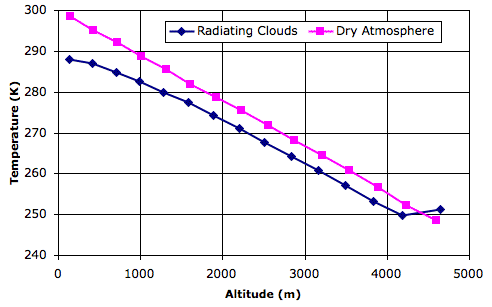
For comparison, we went back to Simulated Planet Surface and loaded the equilibrium state, Day_4, which arises with the same solar heat, but with the surface entirely made of sand. Thus the pink graph shows temperature versus altitude in a dry atmosphere.
The equilibrium state of the dry atmosphere, which looks like this, shows a linear drop in temperature with altitude. According to our calculations, this slope should be −g/Cp, where g is gravity and Cp is the specific heat capacity of the dry gas. Our simulation uses 10 N/kg for gravity and 1003 J/K for Cp, so the slope of the pink graph should be close to −0.010 K/m. Its actual slope is −0.011 K/m.
The equilibrium state of the wet atmosphere, which looks like this, shows a linear drop in temperature only between altitudes 2 km and 4 km. Near the surface of the planet, the heat liberated by condensing water vapor into rising air reduces the amount by which air cools as it rises. In the tropopause, radiation from the planet surface is absorbed by the tropopause clouds, causing them to be warmer than the air immediately below. In the linear region of the graph, the slope is −0.011 K/m, but if we simply divide the total drop in temperature by the altitude of the tropopause, we obtain a net slope of −0.008 K/m.
Looking at graphs such as these, it appears that the Earth's atmosphere has a lapse rate of around −0.0065 K/m. Our simulation does not come up with this lapse rate exactly, but we see that the introduction of water does cause a substantial reduction in the net lapse rate, and with this we are well-satisfied.
The average temperature of the surface of the Earth is around 14°C, or 287 K. This is the average temperature of the air just above the planet surface, not the temperature of the surface itself. The thermometers we use to measure the surface temperature are several meters above the ground. When we use dry air and a sandy surface in our simulation, the average temperature of the surface air is 298 K. But when we add radiating clouds, rain, and snow, the average temperature drops to 288 K, or 15°C. We are well-satisfied with this agreement also.
Sunday, January 22, 2012
Thermal Equillibrium
An object is in thermal equilibrium when the amount of heat entering the object is equal to the amount of heat leaving it. In the case of a planetary system, consisting of a surface and atmosphere, the system will be in thermal equilibrium when the heat arriving from the Sun is, on average, equal to the heat the system radiates into space. The planetary system of our Circulating Cells program will be in thermal equilibrium when the short-wave radiation penetrating to the planet surface from the Sun is balanced by the long-wave radiation escaping into space from its surface, atmospheric gas, clouds, rain, and snow.
When our simulated system converges upon a state where the temperature of its surface and of its atmospheric layers fluctuates around some average value, our hope is that the heat penetrating to the surface from the Sun will be equal, on average, to the heat the system radiates into space. The heat penetrating from the Sun is, of course, the incoming short-wave radiation that is not reflected back into space by our simulated clouds. The heat radiated into space is the upwelling radiation at the top of our simulated atmosphere. We refer to the top of the atmosphere at its tropopause, and to the heat radiated into space as the total escaping power.
We instructed CC11 to print out the average penetrating power from the Sun and the total escaping power from the tropopause every ten hours, and plotted these values for the fourteen thousand hours of the experiment we performed in our previous post. For the final ten thousand hours, the temperature of the surface and the atmospheric layers fluctuate by ±1°C around their average values, as you can see here.

Over the final ten thousand hours, the average penetrating power is 290.0 W/m2 and the average escaping power is 289.6 W/m2. Given the size of the fluctuations in both quantities, and the errors introduced by certain simplifications in our simulation's calculations, we are well-satisfied with this agreement. Our simulation converges upon an equilibrium state that is also a state of thermal equilibrium.
When our simulated system converges upon a state where the temperature of its surface and of its atmospheric layers fluctuates around some average value, our hope is that the heat penetrating to the surface from the Sun will be equal, on average, to the heat the system radiates into space. The heat penetrating from the Sun is, of course, the incoming short-wave radiation that is not reflected back into space by our simulated clouds. The heat radiated into space is the upwelling radiation at the top of our simulated atmosphere. We refer to the top of the atmosphere at its tropopause, and to the heat radiated into space as the total escaping power.
We instructed CC11 to print out the average penetrating power from the Sun and the total escaping power from the tropopause every ten hours, and plotted these values for the fourteen thousand hours of the experiment we performed in our previous post. For the final ten thousand hours, the temperature of the surface and the atmospheric layers fluctuate by ±1°C around their average values, as you can see here.

Over the final ten thousand hours, the average penetrating power is 290.0 W/m2 and the average escaping power is 289.6 W/m2. Given the size of the fluctuations in both quantities, and the errors introduced by certain simplifications in our simulation's calculations, we are well-satisfied with this agreement. Our simulation converges upon an equilibrium state that is also a state of thermal equilibrium.
Wednesday, January 18, 2012
Radiating Clouds
The latest version of Circulating Cells implements the upwelling and downwelling radiation calculations we described in Up and Down Radiation. To run the program, download CC11 and follow the instructions at the top of the code. Clouds absorb and emit long-wave radiation as if they were black bodies. We now set the transparency fraction of our atmospheric gas to 0.5, so that it will be transparent to half the wavelengths in the long-wave spectrum and opaque otherwise. The planet surface can radiate heat directly into space at these transparent wavelengths, as it did in Simulated Planet Surface. But now we have clouds doing the same thing, while at the same time reflecting sunlight back into space.
We begin our simulation with the final state of Simulated Rain, which you will find in SR_1200hr. The initial surface air temperature is 292 K, and cloud depth is 1.5 mm. The following graph shows how air temperature and cloud depth vary in the first two thousand hours.

The following graph shows the first fourteen thousand hours. You will find the final state of the array in RC_14000hr. The average surface air temperature over the final ten thousand hours is 288 K, and the average cloud depth is 0.8 mm.

During the course of these fourteen thousand hours, the distribution of clouds in the atmosphere varies greatly. Sometimes there is a layer of clouds just above the surface of the sea. At other times there are clouds along much of the tropopause. For a view of the final state of the simulation, see here.
As we have discussed many times before, the absorption of long-wave radiation by the atmosphere gives rise to the greenhouse effect. The more opaque the atmosphere, the more heat must be radiated into space by the tropopause instead of the planet surface. In order to radiate more heat, the tropopause must be warmer. If the tropopause is warmer, the planet surface must be warmer too, in order to motivate convection to carry heat to the tropopause. When we change our atmospheric gas from 0% to 50% transparency, we expect the surface temperature drop. And indeed it does: by 4°C.
This cooling of 4°C is, however, far less than the cooling of 31°C we observed when we increased the transparency of our gas from 0% to 50% in the absence of simulated clouds. As we have already discussed, clouds and rain greatly reduce the sensitivity of surface temperature to changes in solar power. Now we find that they also greatly reduce the sensitivity of surface temperature to changes in the transparency of the atmospheric gas.
We begin our simulation with the final state of Simulated Rain, which you will find in SR_1200hr. The initial surface air temperature is 292 K, and cloud depth is 1.5 mm. The following graph shows how air temperature and cloud depth vary in the first two thousand hours.
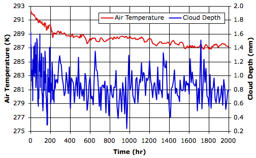
The following graph shows the first fourteen thousand hours. You will find the final state of the array in RC_14000hr. The average surface air temperature over the final ten thousand hours is 288 K, and the average cloud depth is 0.8 mm.
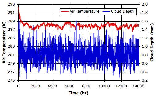
During the course of these fourteen thousand hours, the distribution of clouds in the atmosphere varies greatly. Sometimes there is a layer of clouds just above the surface of the sea. At other times there are clouds along much of the tropopause. For a view of the final state of the simulation, see here.
As we have discussed many times before, the absorption of long-wave radiation by the atmosphere gives rise to the greenhouse effect. The more opaque the atmosphere, the more heat must be radiated into space by the tropopause instead of the planet surface. In order to radiate more heat, the tropopause must be warmer. If the tropopause is warmer, the planet surface must be warmer too, in order to motivate convection to carry heat to the tropopause. When we change our atmospheric gas from 0% to 50% transparency, we expect the surface temperature drop. And indeed it does: by 4°C.
This cooling of 4°C is, however, far less than the cooling of 31°C we observed when we increased the transparency of our gas from 0% to 50% in the absence of simulated clouds. As we have already discussed, clouds and rain greatly reduce the sensitivity of surface temperature to changes in solar power. Now we find that they also greatly reduce the sensitivity of surface temperature to changes in the transparency of the atmospheric gas.
Friday, January 13, 2012
Up and Down Radiation
We are going to add to our Circulating Cells simulation the absorption and emission of long-wave radiation by clouds. As we showed earlier, a liquid water depth of 100 μm absorbs over 99% of all long-wave radiation. Rain contains liquid water also, and ice is a good absorber of long-wave radiation too. We will add the equivalent depth of snow, rain, and cloud droplets for each cell, and so obtain the depth of water within the cell that acts to absorb long-wave radiation.
We note that the same addition of rain, snow, and cloud droplets does not apply to the transmission of short-wave radiation. Water is transparent to short-wave radiation, and clouds reflect it by refracting it through millions of microscopic droplets. But rain and snow contain thousands of times fewer drops and crystals for a given depth of water, so they are thousands of times less effective at refracting sunlight.
For simplicity, we will assume the water in a cell is either transparent or opaque to long-wave radiation, but not in-between. If the combined concentration of rain, snow, and cloud droplets in a cell is greater than wc_opaque, we will assume the entire gas cell is opaque to long-wave radiation. Otherwise, the cell will absorb long-wave radiation as if it were dry, as determined by our transparency_fraction. With our 300-kg cells, a concentration of 0.33 g/kg corresponds to 100 μm of water.
Now we are faced with the possibility of multiple layers of cloud, snow, and rain, all absorbing and emitting long-wave radiation in all directions. The first simplification we make is to assume each gas cell radiates only vertically upwards and downwards. Because our columns of cells are much the same as one another on average, the net effect of this simplification will be small. Even with this simplification, we see that a cloud can absorb radiation from a cloud below, and emit radiation back to that same cloud below, and upwards to a third cloud.
We will calculate the effect of long-wave radiation in the following way. We start at the surface and allow it to radiate as a black body. We allow this upward radiation to enter the first gas cell. We calculate how much is absorbed by the cell and how much keeps going. We calculate how much power the gas cell itself radiates upwards. We add this to the existing upward radiation. We move on to the cell above, and so on, until we get to the tropopause. At the tropopause, we assume the atmosphere above is transparent to long-wave radiation, so all upward-going radiation passes out into space.
We repeat the same process, going down. We start with the tropopause gas cell in each column and move down cell by cell until we arrive at the bottom, at which point all the downward-going radiation is absorbed by the surface. We first considered this kind of downward-going long-wave radiation in our Back Radiation post. It is distinct from the solar radiation that penetrates the atmospheric clouds because it is radiation emitted by the clouds, rain, snow, and atmospheric gas themselves.
In any cell, the long-wave radiation going up is the upwelling radiation and the long-wave radiation going down is the downwelling radiation. At the tropopause, the upwelling radiation is the heat leaving our planetary system. It is our total escaping power. When our simulation converges to equilibrium, we should find that the average solar power penetrating to the surface is equal to the average total escaping power.
We note that the same addition of rain, snow, and cloud droplets does not apply to the transmission of short-wave radiation. Water is transparent to short-wave radiation, and clouds reflect it by refracting it through millions of microscopic droplets. But rain and snow contain thousands of times fewer drops and crystals for a given depth of water, so they are thousands of times less effective at refracting sunlight.
For simplicity, we will assume the water in a cell is either transparent or opaque to long-wave radiation, but not in-between. If the combined concentration of rain, snow, and cloud droplets in a cell is greater than wc_opaque, we will assume the entire gas cell is opaque to long-wave radiation. Otherwise, the cell will absorb long-wave radiation as if it were dry, as determined by our transparency_fraction. With our 300-kg cells, a concentration of 0.33 g/kg corresponds to 100 μm of water.
Now we are faced with the possibility of multiple layers of cloud, snow, and rain, all absorbing and emitting long-wave radiation in all directions. The first simplification we make is to assume each gas cell radiates only vertically upwards and downwards. Because our columns of cells are much the same as one another on average, the net effect of this simplification will be small. Even with this simplification, we see that a cloud can absorb radiation from a cloud below, and emit radiation back to that same cloud below, and upwards to a third cloud.
We will calculate the effect of long-wave radiation in the following way. We start at the surface and allow it to radiate as a black body. We allow this upward radiation to enter the first gas cell. We calculate how much is absorbed by the cell and how much keeps going. We calculate how much power the gas cell itself radiates upwards. We add this to the existing upward radiation. We move on to the cell above, and so on, until we get to the tropopause. At the tropopause, we assume the atmosphere above is transparent to long-wave radiation, so all upward-going radiation passes out into space.
We repeat the same process, going down. We start with the tropopause gas cell in each column and move down cell by cell until we arrive at the bottom, at which point all the downward-going radiation is absorbed by the surface. We first considered this kind of downward-going long-wave radiation in our Back Radiation post. It is distinct from the solar radiation that penetrates the atmospheric clouds because it is radiation emitted by the clouds, rain, snow, and atmospheric gas themselves.
In any cell, the long-wave radiation going up is the upwelling radiation and the long-wave radiation going down is the downwelling radiation. At the tropopause, the upwelling radiation is the heat leaving our planetary system. It is our total escaping power. When our simulation converges to equilibrium, we should find that the average solar power penetrating to the surface is equal to the average total escaping power.
Monday, January 9, 2012
Sinking Restored
When we added rain and snow to our Circulating Cells program, we removed the slow descent of microscopic water droplets, saying that their movement would be insignificant compared with that caused by convection. This is indeed the case when an equilibrium with plenty of atmospheric convection is established.
Nevertheless, we have found in our recent tests, in which we are allowing the clouds to radiate heat directly into space, that clouds can form and sit directly upon the surface, where they block the Sun's light. The surface cools beneath these clouds, and the clouds themselves cool by radiating into space, and we have seen them sit there fore hundreds of hours. This is unrealistic, because in a hundred hours, a cloud will sink by at least a few hundred meters.
So we restored the sinking of cloud droplets to our simulation, at 3 mm/s, which is realistic for cloud droplets 20 μm in diameter.
When we restored the sinking, we noticed that our previous implementation had allowed the clouds to sink only when the cells containing them took part in a convection circulation. As a result, the clouds were sinking through our simulated atmosphere a hundred times slower than they should have been. The fast-sinking implemented by CC9 were in fact sinking at 3 mm/s instead of 300 mm/s, and the slow-sinking clouds were sinking at only 0.03 mm/s instead of 3 mm/s. Thus our fast-sinking clouds were a more realistic simulation of the manner in which actual clouds would sink, while our slow-sinking clouds were unrealistically slow. We run our sinking cloud experiments with a corrected version of CC9, and the new slow-sinking result looked like the former fast-sinking result.
When clouds sink at 3 mm/s, they can sit on the surface for a few hours, but after a hundred hours, they disappear. The droplets will sink 1000 m in a hundred hours, which is three times the height of a gas cells resting upon the surface. The slow descent of the droplets removes clouds that would otherwise freeze the surface, and therefore plays an important role in our simulation, despite the fact that convection, rain, and snow cause movements that are thousands of times faster.
Nevertheless, we have found in our recent tests, in which we are allowing the clouds to radiate heat directly into space, that clouds can form and sit directly upon the surface, where they block the Sun's light. The surface cools beneath these clouds, and the clouds themselves cool by radiating into space, and we have seen them sit there fore hundreds of hours. This is unrealistic, because in a hundred hours, a cloud will sink by at least a few hundred meters.
So we restored the sinking of cloud droplets to our simulation, at 3 mm/s, which is realistic for cloud droplets 20 μm in diameter.
When we restored the sinking, we noticed that our previous implementation had allowed the clouds to sink only when the cells containing them took part in a convection circulation. As a result, the clouds were sinking through our simulated atmosphere a hundred times slower than they should have been. The fast-sinking implemented by CC9 were in fact sinking at 3 mm/s instead of 300 mm/s, and the slow-sinking clouds were sinking at only 0.03 mm/s instead of 3 mm/s. Thus our fast-sinking clouds were a more realistic simulation of the manner in which actual clouds would sink, while our slow-sinking clouds were unrealistically slow. We run our sinking cloud experiments with a corrected version of CC9, and the new slow-sinking result looked like the former fast-sinking result.
When clouds sink at 3 mm/s, they can sit on the surface for a few hours, but after a hundred hours, they disappear. The droplets will sink 1000 m in a hundred hours, which is three times the height of a gas cells resting upon the surface. The slow descent of the droplets removes clouds that would otherwise freeze the surface, and therefore plays an important role in our simulation, despite the fact that convection, rain, and snow cause movements that are thousands of times faster.
Friday, December 23, 2011
Simulated Rain
The latest version of our Circulating Cells program implements the simplified evaporation cycle we presented in our previous post. Freezing clouds turn into snowflakes and drift downwards. When the snowflakes pass through warm air, they melt and become raindrops. To run the program, download CC10 and follow the instructions at the top of the code.
We run the simulation starting with our cold-start state, CS_0hr. The program runs ten times slower than before. The water balancing calculations are more complex now that we have added precipitation, and we must perform them more often because rain and snow move quickly through the atmosphere. Nevertheless, a few hours running gives us six weeks of simulation time, and the atmosphere converges to the equilibrium state shown below, which you will find stored in SR_1200hr. The light gray cells are clouds of water droplets. The white cells are clouds of snowflakes. The dark gray cells are rain.

We see clouds of water droplets in the top row of cells. Here they are cooling by radiation. Our atmosphere is still opaque to long-wave radiation (transparency fraction is zero). Only the top cells can radiate into space. Their temperature is, however, well below 268 K (Tf_droplets), the temperature at which droplets are transformed into ice crystals. Snow forms within the clouds at 0.001 g/kg/s (freeze_rate_gps) and falls at 1 m/s (snow_speed_mps). When it sinks through a cell warmer than 278 K (Tm_ice), it melts at 0.01 g/kg/s (melt_rate_gps), forming rain. Rain falls at 5 m/s (rain_speed_mps).
The following graph shows how surface air temperature and average cloud depth vary with time from our cold start. The final cloud depth fluctuates by ±0.5 mm around an average value of 1.7 mm. The average temperature of the surface gas is 292 K, which is 19°C. Of the light that arrives from the Sun, 30% is reflected into space, giving our simulated planet an albedo of 0.3, which matches that of our own planet Earth.

With fast-sinking clouds, the cloud depth remained close to 2.9 mm and the surface temperature was −7°C. Evaporation from water at 19°C is roughly ten times faster than from from water at −7°C, but precipitation is so effective at removing water from the atmosphere, the sky is almost entirely clear. Indeed, the Sun shines directly upon our island half the time, heating its sandy surface up to 34°C.
We run the simulation starting with our cold-start state, CS_0hr. The program runs ten times slower than before. The water balancing calculations are more complex now that we have added precipitation, and we must perform them more often because rain and snow move quickly through the atmosphere. Nevertheless, a few hours running gives us six weeks of simulation time, and the atmosphere converges to the equilibrium state shown below, which you will find stored in SR_1200hr. The light gray cells are clouds of water droplets. The white cells are clouds of snowflakes. The dark gray cells are rain.
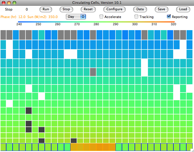
We see clouds of water droplets in the top row of cells. Here they are cooling by radiation. Our atmosphere is still opaque to long-wave radiation (transparency fraction is zero). Only the top cells can radiate into space. Their temperature is, however, well below 268 K (Tf_droplets), the temperature at which droplets are transformed into ice crystals. Snow forms within the clouds at 0.001 g/kg/s (freeze_rate_gps) and falls at 1 m/s (snow_speed_mps). When it sinks through a cell warmer than 278 K (Tm_ice), it melts at 0.01 g/kg/s (melt_rate_gps), forming rain. Rain falls at 5 m/s (rain_speed_mps).
The following graph shows how surface air temperature and average cloud depth vary with time from our cold start. The final cloud depth fluctuates by ±0.5 mm around an average value of 1.7 mm. The average temperature of the surface gas is 292 K, which is 19°C. Of the light that arrives from the Sun, 30% is reflected into space, giving our simulated planet an albedo of 0.3, which matches that of our own planet Earth.
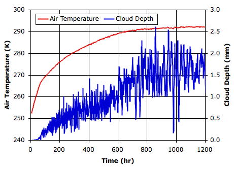
With fast-sinking clouds, the cloud depth remained close to 2.9 mm and the surface temperature was −7°C. Evaporation from water at 19°C is roughly ten times faster than from from water at −7°C, but precipitation is so effective at removing water from the atmosphere, the sky is almost entirely clear. Indeed, the Sun shines directly upon our island half the time, heating its sandy surface up to 34°C.
Monday, December 19, 2011
Evaporation Cycle
The following diagram presents the simplified cycle of evaporation and precipitation we propose to implement in Circulating Cells Version 10.1.

Evaporation takes place from the sea, as before. When a body of moist air rises, it cools, and microscopic droplets form by condensation. Clouds of such droplets that happen to descend from above will warm up, and some or all of their droplets will evaporate. A cloud of droplets whose temperature drops below some threshold Tf will be transformed into snowflakes by the Bergeron Process, warming the surrounding gas with latent heat of fusion. We choose Tf several degrees below the freezing point of water, so we can assume the freezing takes place rapidly.
In our simulation, snow will fall at an average of 1 m/s, which we base upon our own observations. We will implement snow fall in the same way we implemented sinking clouds. Snow that reaches the surface will melt and thus take its latent heat of fusion from the surface block. This melting at the surface is the simplest way we can think of to conserve the latent heat of fusion of the water involved in our evaporation cycle. We assume that our surface water itself never freezes, no matter how cold it gets.
Our clouds, meanwhile, will no longer sink. Real cloud droplets are of order ten microns in diameter and sink at a few millimeters per second. The contribution of such sinking to our new cycle would be negligible.
Snow that enters a gas cell at a temperature greater than Tm will melt, cooling the surrounding gas by absorbing its latent heat of fusion. The melted snowflakes become raindrops a few millimeters in diameter, and these fall at 5 m/s. With the simulation set up as we have it now, the cells are around 400 m high, so rain will take a minute or two to fall out of one cell into the next. We will choose Tm several degrees above the melting point of water so we can assume the melting takes place rapidly.
Our simplified evaporation cycle omits many interesting evaporation-related phenomena. When rain drops are carried up into cold air, for example, they form hail, which later falls to Earth. When liquid rain falls into sufficiently dry air, it evaporates and disappears altogether, giving rise to virga. When air rises at just the right speed along a mountain slope, water droplets join together to form rain drops, as in orographic precipitation. Our simulation will contain none of these interesting phenomena. But we believe it will capture the fundamental features of the Earth's evaporation cycle, and so allow us to investigate how this cycle influences the global surface temperature.
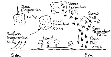
Evaporation takes place from the sea, as before. When a body of moist air rises, it cools, and microscopic droplets form by condensation. Clouds of such droplets that happen to descend from above will warm up, and some or all of their droplets will evaporate. A cloud of droplets whose temperature drops below some threshold Tf will be transformed into snowflakes by the Bergeron Process, warming the surrounding gas with latent heat of fusion. We choose Tf several degrees below the freezing point of water, so we can assume the freezing takes place rapidly.
In our simulation, snow will fall at an average of 1 m/s, which we base upon our own observations. We will implement snow fall in the same way we implemented sinking clouds. Snow that reaches the surface will melt and thus take its latent heat of fusion from the surface block. This melting at the surface is the simplest way we can think of to conserve the latent heat of fusion of the water involved in our evaporation cycle. We assume that our surface water itself never freezes, no matter how cold it gets.
Our clouds, meanwhile, will no longer sink. Real cloud droplets are of order ten microns in diameter and sink at a few millimeters per second. The contribution of such sinking to our new cycle would be negligible.
Snow that enters a gas cell at a temperature greater than Tm will melt, cooling the surrounding gas by absorbing its latent heat of fusion. The melted snowflakes become raindrops a few millimeters in diameter, and these fall at 5 m/s. With the simulation set up as we have it now, the cells are around 400 m high, so rain will take a minute or two to fall out of one cell into the next. We will choose Tm several degrees above the melting point of water so we can assume the melting takes place rapidly.
Our simplified evaporation cycle omits many interesting evaporation-related phenomena. When rain drops are carried up into cold air, for example, they form hail, which later falls to Earth. When liquid rain falls into sufficiently dry air, it evaporates and disappears altogether, giving rise to virga. When air rises at just the right speed along a mountain slope, water droplets join together to form rain drops, as in orographic precipitation. Our simulation will contain none of these interesting phenomena. But we believe it will capture the fundamental features of the Earth's evaporation cycle, and so allow us to investigate how this cycle influences the global surface temperature.
Monday, December 12, 2011
Rain
Our simulated sky never clears. Clouds fill the atmosphere almost entirely. They are forever forming in air that rises from the sea, and forever sinking to the ground, but they never come falling out of the sky all at once in the big drops we know as rain.
The droplets in our clouds are tiny. Those in our slow-sinking clouds are only 10 μm in diameter and descend at 3 mm/s. Those in our fast-sinking clouds descend at 300 mm/s. The graph we present in Falling Droplets implies that these fast-sinking droplets are 100 μm in diameter. Rain falls to Earth at several meters per second, so the same graph tells us that rain drops are at least 500 μm in diameter. A drop 500 μm in diameter contains a hundred times as much water as a droplet of 100 μm and a hundred thousand times as much water as a droplet of 10 μm. Could it be that cloud droplets collide and coalesce in order to form rain drops? If so, how long does this take, and under what circumstances does it occur?
The Wikipedia page on rain describes convective precipitation and orographic precipitation. In both these forms of rain, a cloud moves up, and encounters rain drops descending from above. If the descending drops are 500 μm in diameter, and the air is moving up at 1 m/s, the drops will remain at the same altitude. The cloud moving up and past them carries microscopic droplets that can collide with the stationary drops, coalesce with them, and so enlarge them until they are heavy enough to fall out of the rising cloud and descend to the Earth as rain.
But further reading suggests that rain formed of coalescing droplets is rare. A far more potent source of rain drops are ice crystals. In Cloud Physics, we learn of the Bergeron Process, whereby ice crystals grow, sink, melt, and become rain drops. Large rain-drops are melted hail-stones. Small rain-drops are melted snow-flakes.
In our simulation, whenever the concentration of water vapor exceeds the saturation concentration, we assume the excess water condenses. It turns out, however, that the surface tension of liquid water makes it hard for water to condense into floating, microscopic droplets. If we provide a solid surface for the water to condense against, such as a blade of grass or a glass mirror, the water will condense when it reaches the saturation concentration, but in a body of air high above the ground, the only such surfaces would be dust particles, and these may be rare. Each one will serve as a catalyst for condensation until a droplet forms around it.
But the same is not true of ice crystals. In air saturated with water vapor and below the freezing point of water, an ice crystal can form on a grain of dust, and after that it will continue to grow. Water vapor deposits directly upon the surface of the crystal, thus changing state from gas to solid in one step, and the newly-created ice surface is an ideal foundation for further growth.
Now, suppose a cloud of microscopic water droplets rises until its temperature drops to −20°C. We might assume that the droplets will freeze. But pure water droplets resist freezing until they drop to −40°C. Ice crystals form in the midst of the cloud of super-cooled water droplets. As water vapor is deposited on the crystals, the concentration of water vapor in the air drops.
And here we encounter another curious physical phenomenon. The saturation concentration of water vapor with respect to an ice crystal turns out to be lower than the saturation concentration of water vapor with respect to super-cooled liquid water. Water vapor will deposit on the ice crystals until the concentration of water vapor drops to the saturation concentration of water vapor with respect to ice crystals. Because this concentration is below the saturation concentration with respect to super-cooled liquid water, the water droplets actually start to evaporate. The droplets evaporate, and their water is deposited onto larger and larger ice crystals.
Once the ice crystals are large enough, they start to fall, and they eventually fall into air that is warm enough to melt them. They turn into drops of water and fall to Earth as rain. It is this process that we will attempt to simulate in the next version of our Circulating Cells program.
The droplets in our clouds are tiny. Those in our slow-sinking clouds are only 10 μm in diameter and descend at 3 mm/s. Those in our fast-sinking clouds descend at 300 mm/s. The graph we present in Falling Droplets implies that these fast-sinking droplets are 100 μm in diameter. Rain falls to Earth at several meters per second, so the same graph tells us that rain drops are at least 500 μm in diameter. A drop 500 μm in diameter contains a hundred times as much water as a droplet of 100 μm and a hundred thousand times as much water as a droplet of 10 μm. Could it be that cloud droplets collide and coalesce in order to form rain drops? If so, how long does this take, and under what circumstances does it occur?
The Wikipedia page on rain describes convective precipitation and orographic precipitation. In both these forms of rain, a cloud moves up, and encounters rain drops descending from above. If the descending drops are 500 μm in diameter, and the air is moving up at 1 m/s, the drops will remain at the same altitude. The cloud moving up and past them carries microscopic droplets that can collide with the stationary drops, coalesce with them, and so enlarge them until they are heavy enough to fall out of the rising cloud and descend to the Earth as rain.
But further reading suggests that rain formed of coalescing droplets is rare. A far more potent source of rain drops are ice crystals. In Cloud Physics, we learn of the Bergeron Process, whereby ice crystals grow, sink, melt, and become rain drops. Large rain-drops are melted hail-stones. Small rain-drops are melted snow-flakes.
In our simulation, whenever the concentration of water vapor exceeds the saturation concentration, we assume the excess water condenses. It turns out, however, that the surface tension of liquid water makes it hard for water to condense into floating, microscopic droplets. If we provide a solid surface for the water to condense against, such as a blade of grass or a glass mirror, the water will condense when it reaches the saturation concentration, but in a body of air high above the ground, the only such surfaces would be dust particles, and these may be rare. Each one will serve as a catalyst for condensation until a droplet forms around it.
But the same is not true of ice crystals. In air saturated with water vapor and below the freezing point of water, an ice crystal can form on a grain of dust, and after that it will continue to grow. Water vapor deposits directly upon the surface of the crystal, thus changing state from gas to solid in one step, and the newly-created ice surface is an ideal foundation for further growth.
Now, suppose a cloud of microscopic water droplets rises until its temperature drops to −20°C. We might assume that the droplets will freeze. But pure water droplets resist freezing until they drop to −40°C. Ice crystals form in the midst of the cloud of super-cooled water droplets. As water vapor is deposited on the crystals, the concentration of water vapor in the air drops.
And here we encounter another curious physical phenomenon. The saturation concentration of water vapor with respect to an ice crystal turns out to be lower than the saturation concentration of water vapor with respect to super-cooled liquid water. Water vapor will deposit on the ice crystals until the concentration of water vapor drops to the saturation concentration of water vapor with respect to ice crystals. Because this concentration is below the saturation concentration with respect to super-cooled liquid water, the water droplets actually start to evaporate. The droplets evaporate, and their water is deposited onto larger and larger ice crystals.
Once the ice crystals are large enough, they start to fall, and they eventually fall into air that is warm enough to melt them. They turn into drops of water and fall to Earth as rain. It is this process that we will attempt to simulate in the next version of our Circulating Cells program.
Monday, November 28, 2011
Less Reflection
With 350 W/m2 arriving from the Sun, 75% of the surface covered by water, clouds sinking at 300 mm/s, and each 3 mm of cloud reflecting 63% of sunlight, our CC9 simulation converges upon a surface air temperature of −12°C. When we increase the Sun's power to 400 W/m2, the temperature rises by a mere 0.5°C. Our simulated planet is kept cold by thick clouds that reflect the Sun's light back into space. Ice crystals drift down from the sky in some places, while elsewhere water evaporates from the frozen seas.
The surface of the Earth is at an average temperature well above the freezing point of water, and the Earth's sky is frequently clear of clouds. Our simulated sky never clears, and the surface is frozen. It never rains in our simulation, nor do our simulated clouds emit or absorb radiation. Perhaps these two omissions are responsible for our permanent clouds and frozen seas. Before we attempt to rectify them, however, let us consider the effect of decreasing the reflecting power of our simulated clouds.
We increased Lc_water from 3.0 mm to 6.0 mm, so that it now takes 6.0 mm of cloud water to reflect 63% of the Sun's light. With the reflecting power divided in half, we ran our simulation for eight thousand hours from the starting point CS_0hr. You will find the final state in LR_8000hr.

Compared to before, we now have more clouds in the sky. The following graph shows how cloud depth and surface air temperature vary with time.

Compared to before, we see the atmosphere reaches equilibrium in on third the time. The new temperature is higher and the cloud cover is thicker. The following table compares the state of the atmosphere for both types of clouds.

Our seas are now at −3°C. If they contain salt, they will not freeze. The air a few meters above our sandy island will be just below freezing. Our simulated world is still much colder than the Earth, and nobody standing on the island would ever see the Sun. We are, however, gratified to find that our simulation remains stable with such a large drop in cloud reflectance.
The surface of the Earth is at an average temperature well above the freezing point of water, and the Earth's sky is frequently clear of clouds. Our simulated sky never clears, and the surface is frozen. It never rains in our simulation, nor do our simulated clouds emit or absorb radiation. Perhaps these two omissions are responsible for our permanent clouds and frozen seas. Before we attempt to rectify them, however, let us consider the effect of decreasing the reflecting power of our simulated clouds.
We increased Lc_water from 3.0 mm to 6.0 mm, so that it now takes 6.0 mm of cloud water to reflect 63% of the Sun's light. With the reflecting power divided in half, we ran our simulation for eight thousand hours from the starting point CS_0hr. You will find the final state in LR_8000hr.

Compared to before, we now have more clouds in the sky. The following graph shows how cloud depth and surface air temperature vary with time.
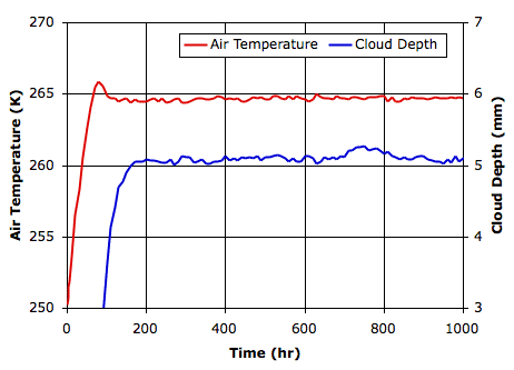
Compared to before, we see the atmosphere reaches equilibrium in on third the time. The new temperature is higher and the cloud cover is thicker. The following table compares the state of the atmosphere for both types of clouds.

Our seas are now at −3°C. If they contain salt, they will not freeze. The air a few meters above our sandy island will be just below freezing. Our simulated world is still much colder than the Earth, and nobody standing on the island would ever see the Sun. We are, however, gratified to find that our simulation remains stable with such a large drop in cloud reflectance.
Subscribe to:
Posts (Atom)