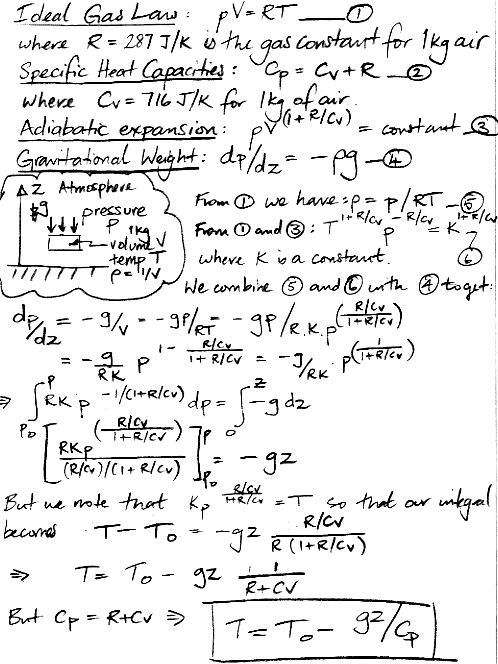
As we saw in Adiabatic Balloons, it takes work to raise gas up from the lower atmosphere. If the temperature of the atmosphere is uniform, the rising gas gets cold as it expands, and is therefore more dense than its surroundings. It tends to sink. At the same time, it takes work to pull gas down from the upper atmosphere. The falling gas gets hot, and is therefore less dense than its surroundings, so it tends to rise.
In Planetary Greenhouse Simulation, we saw what happens when we heat the atmosphere from the bottom, and cool it from the top. The lower atmosphere heats up until a particular temperature profile develops: a linear drop of 50 K from the bottom to the top. Once this profile is established, convection occurs freely. As gas rises, it expands and cools, but the gas around it is already just as cool, so the rising gas continues rising. As gas falls, it compresses and warms, but the gas around it is already just as warm, so the falling gas continues falling. The temperature profile that allows convection is the profile generated by the expansion and compression of circulating gases.
We determined that we could ignore mixing between cells in our simulation. When a volume of gas expands without mixing, it does so according to the equation for adiabatic expansion. In Atmospheric Pressure we calculated pressure as a function of altitude for an atmosphere at constant temperature. Today we calculate pressure as a function of altitude for an atmosphere whose temperature varies with pressure as it would for a dry, ideal, gas expanding adiabatically.

We see that the temperature of an atmosphere stirred by convection must drop linearly with altitude. Michele has proved this to us a number of times, in different ways. The differential form of the result is:
For dry air on Earth, we have g = 10 N/kg and Cp = 1 kJ/kgK, so we expect a drop of 10 K/km. Our simulation uses cells of dry air, and it shows a drop of around 50 K from bottom to top during convection. The temperature drops to 0 K at an altitude zT = CpT0/g. For T0 = 300 K we have zT = 30 km. When the temperature drops to O K, the pressure must be zero also. With a little more pencil-work, we arrive at the following equation for pressure with altitude.
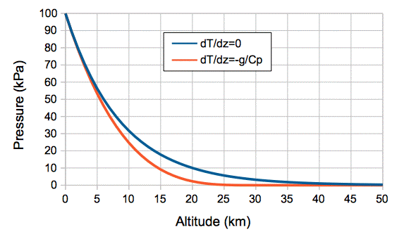
The pressure at the bottom of our cell array is 100 kPa, and at the top is 50 kPa, with the bottom temperature at 300 K. The height of our array is 5.4 km, giving the simulation an average temperature drop of close to 10 K/km. In Atmospheric Pressure, we considered an atmosphere at uniform temperature, and arrived at the relation:
The atmosphere with uniform temperature never comes to a definite end, but keeps getting thinner and thinner with altitude.

Figure: Pressure versus Altitude for Constant Temperature (dT/dz=0) and Adiabatic Convection (dT/dz=−g/Cp) with T0 = 300 K and p0 = 100 kPa. The mass of the atmosphere is p0/g = 10,000 kg/m2 in both cases.
When our cell array is at a uniform temperature T = 250 K, the height of the array will be 5.0 km. Warming the atmosphere to initiate convection causes the top to rise by 400 m.
The −gz/Cp slope of the temperature profile is called the dry adiabatic lapse rate. The Earth's atmosphere is not dry. As moist air expands and cools, water condenses, which releases heat. Thus the wet adiabatic lapse rate is less than the dry adiabatic lapse rate. The lapse rate in the Earth's atmosphere appears to be 6 K/km.
Convection takes place when the temperature drops linearly with altitude. In an atmosphere stirred by convection, gravitational potential and atmospheric temperature are intimately related. A change in one will be matched by an equal and opposite change in the other.

As I showed with the ”(lapse rates of temperatures)” the convection exists also if the lapse rate is not linear.
ReplyDeleteActually, in adiabatic conditions, we have from the momentum equation
δ(u²/2)/δz = - g - Cp*δT/δz + νΔT
a) if Cp*δT/δz > - g + νΔT then the fluid accelerates upward, i.e., it, rising, increases its velocity, falling, decreases its velocity;
b) if Cp*δT/δz = - g + νΔT then the motion of the fluid is uniform
c) Cp*δT/δz < - g + νΔT then the fluid accelerates downward, i.e., it, falling, increases its velocity, rising, decreases its velocity.
The lapse rate alone, according to the thermal diffusion, tells us that
a) if δ²T/δz² > 0 then the fluid gains energy;
b) if δ²T/δz² = 0 then the total energy of the fluid gains is constant;
c) if δ²T/δz² < 0 then the fluid losses energy.
The convection simply takes place when the fluid is no longer at rest and acquires velocity for an acceleration δ(u²/2)/δz thermally induced.
You are right, we are getting closer to understanding the mystery.
Michele
I have extended the height of the atmosphere until 120 km imposing
ReplyDeletea) T = 270 K at 120 km within the thermosphere
b) T = 270 K at 90 km, the top of the stratosphere
c) T = temperature of equilibrium due to the emission 6*T^4 for the thermal sinks of the tropopause at 10 km and the mesopause one at 90 km
d) the same temperatures at the bottom of the troposphere
I have plotted
a) the temperatures ”(temp)”
b) the vertical velocities ”(v)”
c) the vectors of the velocity ”([u,v])”
d) the lapse rates at X15, equator at midday, ”(X15)” , at X22.5 , mid latitude at midday, ”(X22.5)” , at X30, poles, ”(X30)” , at X37.5, mid latitude at mid night, ”(X37.5)” , at X45, equator at midnight, ”(X45)”
FreeFem++ is very powerful.
Michele
Dear Michele,
ReplyDeleteNice work. Why are there three hot spots on the surface for your plot (a). I think I have become confused about the surface heating. You show 0° to 90°, which I assume is pole to equator. What is going on?
I agree with your claims about the lapse rate: higher means the gas will accelerate, which of course means that more heat will be transported, so the bottom will cool, which means the lapse rate will drop.
A lower lapse rate means the gas will slow down, so convection will stop, so the bottom will warm, so the lapse rate will go up.
I conclude that for dry air we should get the adiabatic lapse rate for a wide range of heat flows, and that is what we see in CC5.
Yours, Kevan
Also, see my comment on previous post about your array dimensions. Most convection is in the first 10 km. Your array width is around 100 km. But the circumference of the earth is 40,000 km. So you see circulation that we may not see on Earth. Kevan
ReplyDeleteFirstly in my graphs, the abscissas X represented an Earth’s meridian, longitudinal half of the Earth (from one pole to the other) showed as rectilinear with the following correspondence:
ReplyDelete- daytime: X0/Spole – X15/equator - X30/Npole
- nigthtime: X30/Npole – X45/equator – X60/Spole
but the values obtained at X/0 and X/60 were different although they were referred to the same South Pole at the same time.
The extension of the abscissas until 90 allowed to show once again the daytime side of the same meridian at X60/Spole – X75/equator – X90/Npole, so we obtain a graph perfectly symmetric around X45, with one equator at midnight (X45) and two equators at midday (X15 and X75). Obviously we read only the range between X15 and X75 which represent an entire revolution along the whole meridian midday/midnight with the same values of the parameters at the extremities.
Y-axis represents the height of atmosphere in Km.
The results of my simulation confirm what was well known:
- we need different temperatures on the surface for to activate circulation induced by convection
- the turbulence is present almost exclusively within the lowest region of the tropopause
- if the Earth is not rotating in the space, without the Coriolis forces, the global circulation occurs according to a simplified one-cell way between the equator and the poles, as we can see, e.g., at http://www.physicalgeography.net/fundamentals/7p.html or at many other sites of physical geography on the web.
Michele
"errata corrige"
ReplyDeletetropopause >>>> troposphere
Michele
Dear Michele,
ReplyDeleteThanks for your explanation. I understand the plots now. They would be clearer is your used latitude for your x-axis, so the equators would be at 90, 270, and 450 degrees.
I will go back and look at the comment where you explain the way you heat the air at the surface. I think you use constant-temperature, with the night-time equator being cooler than the day-time equator.
I agree that there is a net circulation observed on Earth and Venus of gases rising at the equator and moving towards the poles. But so far as I can tell, the velocity is small compared to the local convection and wind that occurs on Earth. Most convection is local.
What do you have to say about the scale of the x-axis compared to the y-axis? On Earth, the atmosphere is a thin skin. In your plot, it is a thick layer.
Yours, Kevan
The temperature at ground are shown here. ”(Temperatures)”
ReplyDeleteThe velocities of the graphs are km/s.
The horizontal scale is more smaller than the vertical for to show well what occurs. Whit the same scale one could view nothing.
Michele
I see, so you are saying that the horizontal axis represents 40,000 km from x=0 to x=60, is that right? Yours, Kevan
ReplyDeleteYes, that's right.
ReplyDeleteMichele
I see: so these circulations do indeed occur from equator to pole. I think they are called Hadley Cells. In your vertical velocity plot, what is the scale? What does velocity 0.001 represent? What is the horizontal velocity of this circulation?
ReplyDeleteI have performed my calculations using the km as unity of measure of the lengths and I have not introduced any correction to take into account that 60 unities of abscissa correspond to 40,000 km. Thus, whereas the used vertical gradients are real, the horizontal ones are more stronger. If that doesn’t affect the results, the vertical speeds must have to be multiplied by 1000 and the horizontal ones by 6.67E5 to obtain the velocity in m/s. I don’t know how/if is it possible to use different scales for X and Y using FreeFem++, I will investigate for.
ReplyDeleteMy first idea was to get a qualitative reading of what happens in the atmosphere and above all to see the macro/micro turbulences, getting the interesting result that the micro turbulences abut on the peripheral regions in proximity of the walls and that only one macro turbulence is gotten for every inclusive region among the equator and the poles, that’s exactly the Hadley Cell.
Michele
Dear Michele,
ReplyDeleteI"m looking at your velocity vector plot here and comparing it to your vertical velocity plot here to estimate the horizontal component of velocity. I see vectors at 45° combined with velocity of 0.002, which implies a horizontal component of order 0.001. If I multiply by 670,000 m/s I get 670 m/s for the horizontal component, which is twice the speed of sound.
What am I missing here? Perhaps you could plot the horizontal velocity directly. The velocity should be a hundred times smaller, or ten thousand times less energetic.
Yours, Kevan
I have simply multiplied by 1000 both u and v obtaining values very believable.
ReplyDelete”(umod)”
”(vmod)”
If I will be able to do it, I will verify the PDE system for to test if it is dimensionally consistent.
Michele