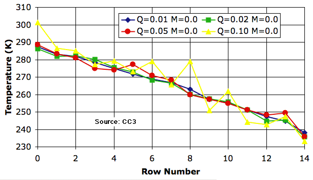
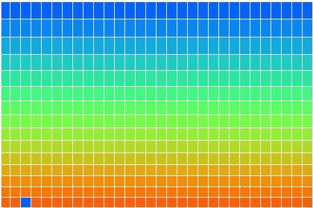
The anthropogenic global warming (AGW) hypothesis presented by the majority of today's climatologists has two parts. First it claims that the world is getting exceptionally warm, and second it claims that human carbon dioxide (CO2) emissions are the cause of this warming. Seven years ago, we began our personal investigation of this hypothesis, and we did so by considering whether or not the world was indeed getting exceptionally warm.
The first thing we did was estimate the uncertainty inherent in the measurements of global surface temperature. We concluded that natural variations in local climate introduce an error of roughly 0.14°C in the measurement of the change in temperature between any two points in time. The fact that the error is constant with the time over which we measure the change is a consequence of the particular characteristics of local climate fluctuations.
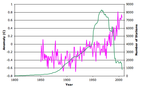
We downloaded the weather station data from NCDC and calculated the global surface anomaly using a method we called integrated derivatives, but which others have called first differences. The graph we obtained was almost identical to the one obtained by CRU using their complex reference grid method. It remains a mystery to us why institutions like CRU, NASA, and NCDC use such a complex method when a far simpler one will do. All graphs show roughly a 0.6°C rise in global surface temperature from 1950 to 2000. This rise is significant compared to our expected resolution of 0.14°C.
We made this plot superimposing the number of weather stations and the global surface anomaly versus time. The number of weather stations drops dramatically from 1960 and 1990. Only one in four remain active at the end of this thirty-year period. During the same period, the global surface anomaly shows a 0.6°C rise. By selecting subsets of the weather stations, we found that the apparent warming from 1950 to 1990 varied from 0.3°C to 1.0°C depending upon whether we used stations that disappeared in that period, persisted through that period, or existed shorter or longer intervals in the same century. Thus is seemed to us that some significant amount of work would have to be done to eliminate the change in the number of weather stations as a source of error in the data. But we saw no mention whatsoever of this source of error in published papers in which the global surface anomaly is presented, such as Jones et al..
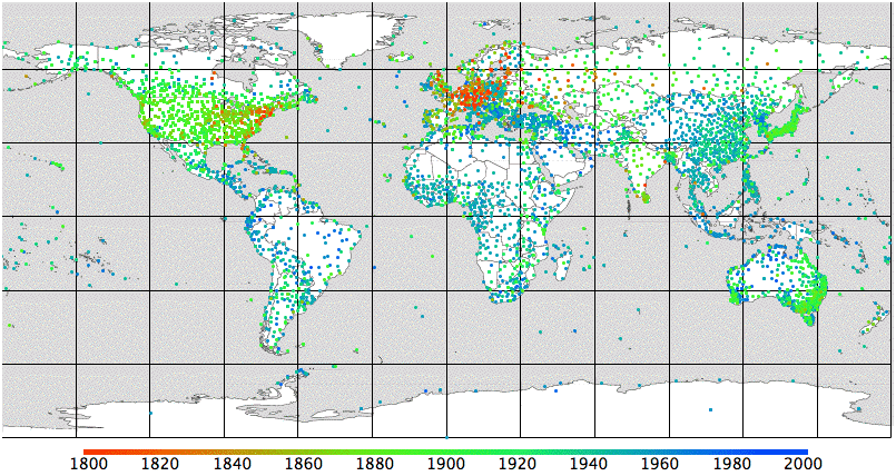
We plotted a global map of the available weather stations, color-coded to show the date they first started reporting. The map shows that almost all stations in the tropics began operating after 1930, while most of those in the temperate regions were operating by 1880. This seems to us to be another source of systematic error in our measurement of the global surface anomaly.
Weather stations might also be affected by the appearance of buildings, tarmac, and road traffic. We found examples of weather stations in which such urban heating caused an apparent warming of several degrees centigrade over a few decades. It seemed to us that this effect would have to be examined in depth by any paper presenting a global surface trend. But papers such as Jones et al. do not address the urban heating issue directly. Instead, they claim that the effect is negligible and refer to other papers as proof. But when we looked up those other papers, we did not find any such proof.
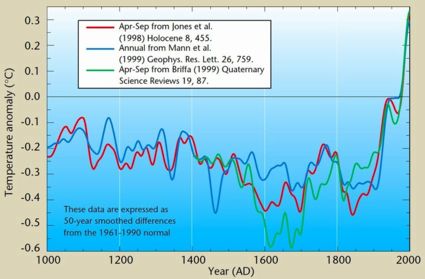
In order to argue that modern temperatures were exceptionally warm, climatologists produced the hockey stick graph, in which a collection of potential long-term measurements of global surface temperature were combined together under the assumption that they could be trusted only to the extent that they showed a temperatures increase from 1950 to 2000. Indeed, if a measurement showed a temperature decline in that period, the hockey stick method would flip the trend over and add it to the combination so that it now contributed to a rise in the same period.
The hockey-stick graph shows no sign of the Medieval Warm Period, in which Greenland was inhabited by farmers, nor the Little Ice Age, when the Thames was known to freeze over, and nor should we expect it to. Given a random set of measurements, the hockey-stick combination method will almost always produce a graph that shows a sharp rise from 1950 to 2000 and a gentle descent during the thousand years before-hand. When applied to the existing measurements of temperature by tree rings, ice cores, and other such indirect methods, it is no surprise that the method produced that same shape.
We presented our doubts about the surface temperature measurements and the hockey stick graph to believers in the AGW hypothesis. We were received with disdain and given no satisfactory answers. Furthermore, the Climategate affair revealed several significant breaches of scientific method by the climate science community. For example, in this graph produced by climatologists for the World Health Organization, the authors removed the tree ring temperature data from 1960 onwards because it showed a decline in temperature, and substituted temperature station measurements in their place. They plotted the combination as a single line. When I asked a prominent climatologists what exactly had been done, he said, "The smooth was calculated using instrumental data past 1960." He declared that a better way to handle the divergence of the tree-ring data from the station measurements would be to cut short the graph of tree-ring data at 1960, so as to hide the decline in temperatures measured by the tree rings.
What we see here is the assumption by climatologists that the world has been warming up and that the global temperature measured by weather stations is correct. This assumption leads them to delete conflicting data on the grounds that it must be bad data. Thus it becomes impossible for them to discover that their assumption is incorrect. By this time, we were skeptical of the global surface anomaly we obtained from the station data. We were no longer certain that the data itself had not been modified by NCDC. We had little reason to trust any other measurement produced by climatologists, we were unimpressed with the hockey-stick method of combining measurements, and we were quite certain that recent temperatures were not exceptional for the past ten thousand years.
We turned our attention to the second part of the AGW hypothesis: the one that says doubling the atmosphere's CO2 concentration will increase the surface temperature by roughly 3°C. It took us a long time to come to a conclusion on this one. The climate models upon which such predictions are based are private property of various climatologists. In any event, we do not trust models produced by a community that is willing to delete data that conflict with its assumptions. If they are willing to delete data, we must assume that they are willing to adjust their models until the models give predictions consistent with their AGW hypothesis.
We began with some laboratory experiments on radiation. We stated the principle of the greenhouse effect. After a great deal of searching around, we eventually obtained the absorption spectrum of various layers of the Earth's atmosphere. This allowed us to confirm that, if the skies remained clear, a doubling of CO2 concentration would cause the world to warm up by about 1.5°C.
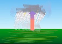
But of course the skies don't remain clear. The formation of clouds is a strong function of surface temperature. If the world warms up, there will be more clouds. They will reflect more of the Sun's light, while at the same time, slowing down the radiation of heat into space by the Earth. To determine how these two effects would interact, we built our own climate model, which we called Circulating Cells.
When it comes to determining the effect of increased cloud cover, the most critical parameter to decide upon is the reflection of sunlight by clouds per millimeter of water depth in the cloud. It seemed to us that there should be a large body of literature written recently upon this subject because it is so important to climate modeling. The best paper we found upon the subject was written in 1948, Reflection, Absorption, and Transmission of Insolation by Stratus Cloud. We found a couple of more recent papers about reflection, such as this one, but they do not attempt to provide an empirical formula for the reflection of clouds with increasing cloud depth. We concluded that climatologists are not examining this issue in detail.
In a long sequence of small steps, we built up our climate model until it implemented surface convection, surface heat capacity, evaporation, cloud formation, precipitation, and radiation by clouds. We tested every aspect of the simulation in detail, and based its operating parameters upon our own estimates and upon whatever measurements we could find in climate science journals. We did not choose our model parameters to suit any hypothesis of our own, nor could we have done, because we did not have a model capable of testing the AGW hypothesis until the final stage, and we did not change the parameters in that final stage.
The latest version of our climate model shows that cloud cover increases rapidly as the surface warms above the freezing point of water. The evaporation rate of water from the surface increases approximately as the square of the temperature above freezing, and the only way for water to return to the surface is to form a cloud first. If we ignore the increased reflection of sunlight due to increasing cloud cover, and consider only the slowing-down of radiation into space by the same increase in cloud cover, our model shows roughly 3°C of warming due to a doubling in CO2 concentration. But when we take account of the increased reflection of sunlight by the increasing cloud cover, the warming drops to 0.9°C.
It seems to us that the climate models used by climatologists ignore the reflection of sunlight due to clouds. They may allow for some fixed fraction of sunlight to be reflected by clouds, but they do not allow this fraction to increase with increasing surface temperature. Thus they conclude that the warming due to CO2 doubling will be 3°C. If they took account of the increased reflection, the effect would be far smaller and less dramatic: roughly 1°C.
Doubling the CO2 concentration of the atmosphere will indeed encourage the world to warm up, but not by enough that we should worry. Right now CO2 concentration has increased from roughly 300 ppm to 400 ppm in the past century. If it gets to 600 ppm then we can say that the rise in CO2 concentration will tend to warm the Earth by 1°C. But we are unlikely to be able to check our calculations, because the natural variation in the Earth's climate is itself of order ±1°C from one century to the next.
And so we find ourselves at the end of our journey. Modern warming is not exceptional, and doubling the CO2 concentration will cause the world to warm up by roughly 1°C, not 3°C. The only part of the AGW theory we have not investigated is its assertion that human CO2 emissions are responsible for the increase in atmospheric CO2 concentration over the past century.
My thanks to those of you who took part in the effort, both by private e-mails and in the comments. I would not have continued the effort without your participation. I hope it is clear that my use of "we" instead of "I" is in recognition of the fact that this has been a group effort. I will continue to answer comments on this site, and I will consider any suggestions of further work. To the first approximation, however: we're done.
Showing posts with label Weather. Show all posts
Showing posts with label Weather. Show all posts
Wednesday, April 4, 2012


Friday, December 23, 2011
Simulated Rain
The latest version of our Circulating Cells program implements the simplified evaporation cycle we presented in our previous post. Freezing clouds turn into snowflakes and drift downwards. When the snowflakes pass through warm air, they melt and become raindrops. To run the program, download CC10 and follow the instructions at the top of the code.
We run the simulation starting with our cold-start state, CS_0hr. The program runs ten times slower than before. The water balancing calculations are more complex now that we have added precipitation, and we must perform them more often because rain and snow move quickly through the atmosphere. Nevertheless, a few hours running gives us six weeks of simulation time, and the atmosphere converges to the equilibrium state shown below, which you will find stored in SR_1200hr. The light gray cells are clouds of water droplets. The white cells are clouds of snowflakes. The dark gray cells are rain.

We see clouds of water droplets in the top row of cells. Here they are cooling by radiation. Our atmosphere is still opaque to long-wave radiation (transparency fraction is zero). Only the top cells can radiate into space. Their temperature is, however, well below 268 K (Tf_droplets), the temperature at which droplets are transformed into ice crystals. Snow forms within the clouds at 0.001 g/kg/s (freeze_rate_gps) and falls at 1 m/s (snow_speed_mps). When it sinks through a cell warmer than 278 K (Tm_ice), it melts at 0.01 g/kg/s (melt_rate_gps), forming rain. Rain falls at 5 m/s (rain_speed_mps).
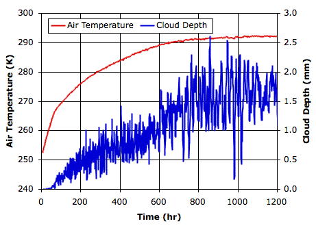
The following graph shows how surface air temperature and average cloud depth vary with time from our cold start. The final cloud depth fluctuates by ±0.5 mm around an average value of 1.7 mm. The average temperature of the surface gas is 292 K, which is 19°C. Of the light that arrives from the Sun, 30% is reflected into space, giving our simulated planet an albedo of 0.3, which matches that of our own planet Earth.

With fast-sinking clouds, the cloud depth remained close to 2.9 mm and the surface temperature was −7°C. Evaporation from water at 19°C is roughly ten times faster than from from water at −7°C, but precipitation is so effective at removing water from the atmosphere, the sky is almost entirely clear. Indeed, the Sun shines directly upon our island half the time, heating its sandy surface up to 34°C.
We run the simulation starting with our cold-start state, CS_0hr. The program runs ten times slower than before. The water balancing calculations are more complex now that we have added precipitation, and we must perform them more often because rain and snow move quickly through the atmosphere. Nevertheless, a few hours running gives us six weeks of simulation time, and the atmosphere converges to the equilibrium state shown below, which you will find stored in SR_1200hr. The light gray cells are clouds of water droplets. The white cells are clouds of snowflakes. The dark gray cells are rain.
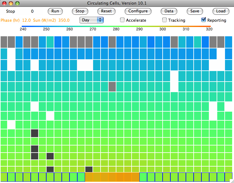
We see clouds of water droplets in the top row of cells. Here they are cooling by radiation. Our atmosphere is still opaque to long-wave radiation (transparency fraction is zero). Only the top cells can radiate into space. Their temperature is, however, well below 268 K (Tf_droplets), the temperature at which droplets are transformed into ice crystals. Snow forms within the clouds at 0.001 g/kg/s (freeze_rate_gps) and falls at 1 m/s (snow_speed_mps). When it sinks through a cell warmer than 278 K (Tm_ice), it melts at 0.01 g/kg/s (melt_rate_gps), forming rain. Rain falls at 5 m/s (rain_speed_mps).
The following graph shows how surface air temperature and average cloud depth vary with time from our cold start. The final cloud depth fluctuates by ±0.5 mm around an average value of 1.7 mm. The average temperature of the surface gas is 292 K, which is 19°C. Of the light that arrives from the Sun, 30% is reflected into space, giving our simulated planet an albedo of 0.3, which matches that of our own planet Earth.
With fast-sinking clouds, the cloud depth remained close to 2.9 mm and the surface temperature was −7°C. Evaporation from water at 19°C is roughly ten times faster than from from water at −7°C, but precipitation is so effective at removing water from the atmosphere, the sky is almost entirely clear. Indeed, the Sun shines directly upon our island half the time, heating its sandy surface up to 34°C.
Monday, December 19, 2011
Evaporation Cycle
The following diagram presents the simplified cycle of evaporation and precipitation we propose to implement in Circulating Cells Version 10.1.

Evaporation takes place from the sea, as before. When a body of moist air rises, it cools, and microscopic droplets form by condensation. Clouds of such droplets that happen to descend from above will warm up, and some or all of their droplets will evaporate. A cloud of droplets whose temperature drops below some threshold Tf will be transformed into snowflakes by the Bergeron Process, warming the surrounding gas with latent heat of fusion. We choose Tf several degrees below the freezing point of water, so we can assume the freezing takes place rapidly.
In our simulation, snow will fall at an average of 1 m/s, which we base upon our own observations. We will implement snow fall in the same way we implemented sinking clouds. Snow that reaches the surface will melt and thus take its latent heat of fusion from the surface block. This melting at the surface is the simplest way we can think of to conserve the latent heat of fusion of the water involved in our evaporation cycle. We assume that our surface water itself never freezes, no matter how cold it gets.
Our clouds, meanwhile, will no longer sink. Real cloud droplets are of order ten microns in diameter and sink at a few millimeters per second. The contribution of such sinking to our new cycle would be negligible.
Snow that enters a gas cell at a temperature greater than Tm will melt, cooling the surrounding gas by absorbing its latent heat of fusion. The melted snowflakes become raindrops a few millimeters in diameter, and these fall at 5 m/s. With the simulation set up as we have it now, the cells are around 400 m high, so rain will take a minute or two to fall out of one cell into the next. We will choose Tm several degrees above the melting point of water so we can assume the melting takes place rapidly.
Our simplified evaporation cycle omits many interesting evaporation-related phenomena. When rain drops are carried up into cold air, for example, they form hail, which later falls to Earth. When liquid rain falls into sufficiently dry air, it evaporates and disappears altogether, giving rise to virga. When air rises at just the right speed along a mountain slope, water droplets join together to form rain drops, as in orographic precipitation. Our simulation will contain none of these interesting phenomena. But we believe it will capture the fundamental features of the Earth's evaporation cycle, and so allow us to investigate how this cycle influences the global surface temperature.
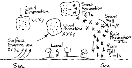
Evaporation takes place from the sea, as before. When a body of moist air rises, it cools, and microscopic droplets form by condensation. Clouds of such droplets that happen to descend from above will warm up, and some or all of their droplets will evaporate. A cloud of droplets whose temperature drops below some threshold Tf will be transformed into snowflakes by the Bergeron Process, warming the surrounding gas with latent heat of fusion. We choose Tf several degrees below the freezing point of water, so we can assume the freezing takes place rapidly.
In our simulation, snow will fall at an average of 1 m/s, which we base upon our own observations. We will implement snow fall in the same way we implemented sinking clouds. Snow that reaches the surface will melt and thus take its latent heat of fusion from the surface block. This melting at the surface is the simplest way we can think of to conserve the latent heat of fusion of the water involved in our evaporation cycle. We assume that our surface water itself never freezes, no matter how cold it gets.
Our clouds, meanwhile, will no longer sink. Real cloud droplets are of order ten microns in diameter and sink at a few millimeters per second. The contribution of such sinking to our new cycle would be negligible.
Snow that enters a gas cell at a temperature greater than Tm will melt, cooling the surrounding gas by absorbing its latent heat of fusion. The melted snowflakes become raindrops a few millimeters in diameter, and these fall at 5 m/s. With the simulation set up as we have it now, the cells are around 400 m high, so rain will take a minute or two to fall out of one cell into the next. We will choose Tm several degrees above the melting point of water so we can assume the melting takes place rapidly.
Our simplified evaporation cycle omits many interesting evaporation-related phenomena. When rain drops are carried up into cold air, for example, they form hail, which later falls to Earth. When liquid rain falls into sufficiently dry air, it evaporates and disappears altogether, giving rise to virga. When air rises at just the right speed along a mountain slope, water droplets join together to form rain drops, as in orographic precipitation. Our simulation will contain none of these interesting phenomena. But we believe it will capture the fundamental features of the Earth's evaporation cycle, and so allow us to investigate how this cycle influences the global surface temperature.
Monday, December 12, 2011
Rain
Our simulated sky never clears. Clouds fill the atmosphere almost entirely. They are forever forming in air that rises from the sea, and forever sinking to the ground, but they never come falling out of the sky all at once in the big drops we know as rain.
The droplets in our clouds are tiny. Those in our slow-sinking clouds are only 10 μm in diameter and descend at 3 mm/s. Those in our fast-sinking clouds descend at 300 mm/s. The graph we present in Falling Droplets implies that these fast-sinking droplets are 100 μm in diameter. Rain falls to Earth at several meters per second, so the same graph tells us that rain drops are at least 500 μm in diameter. A drop 500 μm in diameter contains a hundred times as much water as a droplet of 100 μm and a hundred thousand times as much water as a droplet of 10 μm. Could it be that cloud droplets collide and coalesce in order to form rain drops? If so, how long does this take, and under what circumstances does it occur?
The Wikipedia page on rain describes convective precipitation and orographic precipitation. In both these forms of rain, a cloud moves up, and encounters rain drops descending from above. If the descending drops are 500 μm in diameter, and the air is moving up at 1 m/s, the drops will remain at the same altitude. The cloud moving up and past them carries microscopic droplets that can collide with the stationary drops, coalesce with them, and so enlarge them until they are heavy enough to fall out of the rising cloud and descend to the Earth as rain.
But further reading suggests that rain formed of coalescing droplets is rare. A far more potent source of rain drops are ice crystals. In Cloud Physics, we learn of the Bergeron Process, whereby ice crystals grow, sink, melt, and become rain drops. Large rain-drops are melted hail-stones. Small rain-drops are melted snow-flakes.
In our simulation, whenever the concentration of water vapor exceeds the saturation concentration, we assume the excess water condenses. It turns out, however, that the surface tension of liquid water makes it hard for water to condense into floating, microscopic droplets. If we provide a solid surface for the water to condense against, such as a blade of grass or a glass mirror, the water will condense when it reaches the saturation concentration, but in a body of air high above the ground, the only such surfaces would be dust particles, and these may be rare. Each one will serve as a catalyst for condensation until a droplet forms around it.
But the same is not true of ice crystals. In air saturated with water vapor and below the freezing point of water, an ice crystal can form on a grain of dust, and after that it will continue to grow. Water vapor deposits directly upon the surface of the crystal, thus changing state from gas to solid in one step, and the newly-created ice surface is an ideal foundation for further growth.
Now, suppose a cloud of microscopic water droplets rises until its temperature drops to −20°C. We might assume that the droplets will freeze. But pure water droplets resist freezing until they drop to −40°C. Ice crystals form in the midst of the cloud of super-cooled water droplets. As water vapor is deposited on the crystals, the concentration of water vapor in the air drops.
And here we encounter another curious physical phenomenon. The saturation concentration of water vapor with respect to an ice crystal turns out to be lower than the saturation concentration of water vapor with respect to super-cooled liquid water. Water vapor will deposit on the ice crystals until the concentration of water vapor drops to the saturation concentration of water vapor with respect to ice crystals. Because this concentration is below the saturation concentration with respect to super-cooled liquid water, the water droplets actually start to evaporate. The droplets evaporate, and their water is deposited onto larger and larger ice crystals.
Once the ice crystals are large enough, they start to fall, and they eventually fall into air that is warm enough to melt them. They turn into drops of water and fall to Earth as rain. It is this process that we will attempt to simulate in the next version of our Circulating Cells program.
The droplets in our clouds are tiny. Those in our slow-sinking clouds are only 10 μm in diameter and descend at 3 mm/s. Those in our fast-sinking clouds descend at 300 mm/s. The graph we present in Falling Droplets implies that these fast-sinking droplets are 100 μm in diameter. Rain falls to Earth at several meters per second, so the same graph tells us that rain drops are at least 500 μm in diameter. A drop 500 μm in diameter contains a hundred times as much water as a droplet of 100 μm and a hundred thousand times as much water as a droplet of 10 μm. Could it be that cloud droplets collide and coalesce in order to form rain drops? If so, how long does this take, and under what circumstances does it occur?
The Wikipedia page on rain describes convective precipitation and orographic precipitation. In both these forms of rain, a cloud moves up, and encounters rain drops descending from above. If the descending drops are 500 μm in diameter, and the air is moving up at 1 m/s, the drops will remain at the same altitude. The cloud moving up and past them carries microscopic droplets that can collide with the stationary drops, coalesce with them, and so enlarge them until they are heavy enough to fall out of the rising cloud and descend to the Earth as rain.
But further reading suggests that rain formed of coalescing droplets is rare. A far more potent source of rain drops are ice crystals. In Cloud Physics, we learn of the Bergeron Process, whereby ice crystals grow, sink, melt, and become rain drops. Large rain-drops are melted hail-stones. Small rain-drops are melted snow-flakes.
In our simulation, whenever the concentration of water vapor exceeds the saturation concentration, we assume the excess water condenses. It turns out, however, that the surface tension of liquid water makes it hard for water to condense into floating, microscopic droplets. If we provide a solid surface for the water to condense against, such as a blade of grass or a glass mirror, the water will condense when it reaches the saturation concentration, but in a body of air high above the ground, the only such surfaces would be dust particles, and these may be rare. Each one will serve as a catalyst for condensation until a droplet forms around it.
But the same is not true of ice crystals. In air saturated with water vapor and below the freezing point of water, an ice crystal can form on a grain of dust, and after that it will continue to grow. Water vapor deposits directly upon the surface of the crystal, thus changing state from gas to solid in one step, and the newly-created ice surface is an ideal foundation for further growth.
Now, suppose a cloud of microscopic water droplets rises until its temperature drops to −20°C. We might assume that the droplets will freeze. But pure water droplets resist freezing until they drop to −40°C. Ice crystals form in the midst of the cloud of super-cooled water droplets. As water vapor is deposited on the crystals, the concentration of water vapor in the air drops.
And here we encounter another curious physical phenomenon. The saturation concentration of water vapor with respect to an ice crystal turns out to be lower than the saturation concentration of water vapor with respect to super-cooled liquid water. Water vapor will deposit on the ice crystals until the concentration of water vapor drops to the saturation concentration of water vapor with respect to ice crystals. Because this concentration is below the saturation concentration with respect to super-cooled liquid water, the water droplets actually start to evaporate. The droplets evaporate, and their water is deposited onto larger and larger ice crystals.
Once the ice crystals are large enough, they start to fall, and they eventually fall into air that is warm enough to melt them. They turn into drops of water and fall to Earth as rain. It is this process that we will attempt to simulate in the next version of our Circulating Cells program.
Tuesday, November 15, 2011
Fast-Sinking Clouds
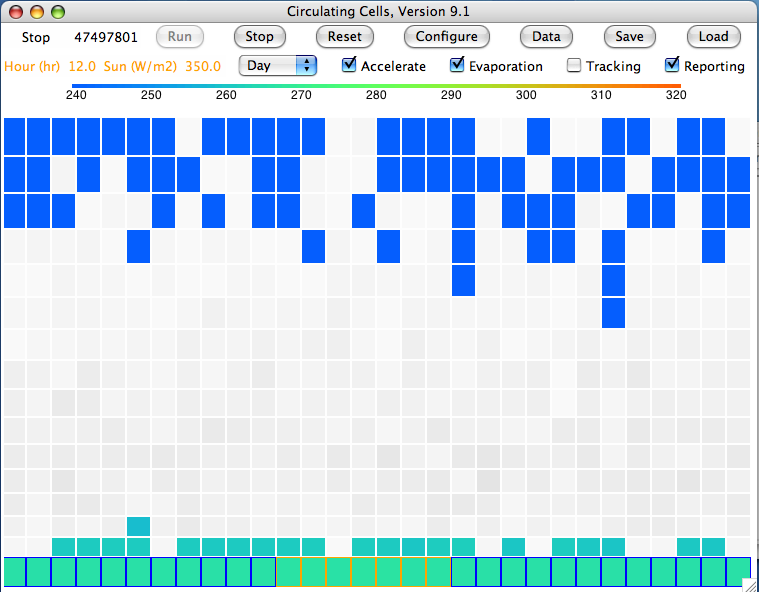
In our previous post we allowed the clouds in our simulation to sink to the surface at 3 mm/s. We implemented this sinking by allowing an average of 0.001% of each cell's water droplets to drop down out of the cell every second (0.1% every 100 s). Today we repeat our experiment from the same starting point, but this time the gas cells lose 0.1% of their water droplets per second, which corresponds to droplets sinking at 300 mm/s. Here is the state of the atmosphere after thirteen thousand hours.

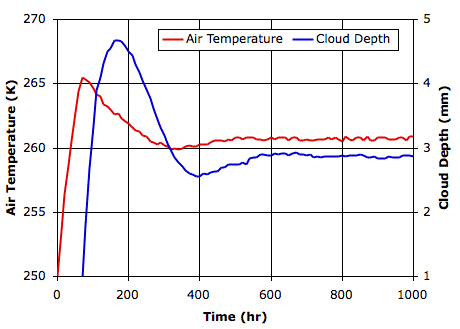
Although our screen shot is taken at thirteen thousand hours, the atmosphere converges to its equilibrium state in a mere eight hundred hours. Our previous simulation converged only after eight thousand hours. The following graph shows surface gas temperature and cloud depth versus time.

The following table compares the equilibrium state of the atmosphere at the end of our two experiments.

The faster-sinking clouds cause the surface to warm by 5.3 K. The Solar power penetrating to the surface increases by 13 W/m2 because the clouds are slightly thinner. You may recall that our current simulation of clouds does not implement their absorption and emission of long-wave radiation, so we are working with transparency fraction set to 0.0, indicating an atmospheric gas that is opaque to long-wave radiation. The only place for this artificial atmosphere to radiate is at the tropopause. So we expect to see the tropopause radiating the same amount of heat that penetrates to the surface: the heat leaving the system must be equal to the heat entering. And indeed this is the case to within a couple of Watts per square meter.
We see that faster-sinking clouds cause the world to warm up, and this is in keeping with our expectation. The icy surface must warm up so that evaporation will keep up with the greater rate of return of water to the surface.
UPDATE: It turns out that our code was allowing clouds to sink only when they took part in a circulation, which resulted in them sinking roughly a hundred times slower than they should have, so our effective sinking rate here was more like 3 mm/s. When we correct our error, so that the clouds really do sink at 300 mm/s, the surface temperature warms by roughly 7 K. [07-JAN-12]
Although our screen shot is taken at thirteen thousand hours, the atmosphere converges to its equilibrium state in a mere eight hundred hours. Our previous simulation converged only after eight thousand hours. The following graph shows surface gas temperature and cloud depth versus time.
The following table compares the equilibrium state of the atmosphere at the end of our two experiments.

The faster-sinking clouds cause the surface to warm by 5.3 K. The Solar power penetrating to the surface increases by 13 W/m2 because the clouds are slightly thinner. You may recall that our current simulation of clouds does not implement their absorption and emission of long-wave radiation, so we are working with transparency fraction set to 0.0, indicating an atmospheric gas that is opaque to long-wave radiation. The only place for this artificial atmosphere to radiate is at the tropopause. So we expect to see the tropopause radiating the same amount of heat that penetrates to the surface: the heat leaving the system must be equal to the heat entering. And indeed this is the case to within a couple of Watts per square meter.
We see that faster-sinking clouds cause the world to warm up, and this is in keeping with our expectation. The icy surface must warm up so that evaporation will keep up with the greater rate of return of water to the surface.
UPDATE: It turns out that our code was allowing clouds to sink only when they took part in a circulation, which resulted in them sinking roughly a hundred times slower than they should have, so our effective sinking rate here was more like 3 mm/s. When we correct our error, so that the clouds really do sink at 300 mm/s, the surface temperature warms by roughly 7 K. [07-JAN-12]
Friday, November 11, 2011
Slow-Sinking Clouds
In Falling Droplets, we concluded that 10-μm water droplets will sink at 3 mm/s in air at pressure 100 kPa. The lowest atmospheric cells in our Circulating Cells program are at 100 kPa, and they are roughly 300 m high, so we see that it will take a hundred thousand seconds for a droplet to fall the height of the cell. Cells higher up are taller, but the gas within them is thinner. A droplet must fall more quickly through thinner air before its weight is matched by air resistance. For simplicity, we will assume that the time it takes a 10-μm droplet to fall the height of a cell is the same regardless of altitude.
As we found in Simulation Time, our program checks each gas cell every one hundred iterations on average, which corresponds to every 100 s. If it takes a droplet one hundred thousand seconds to fall the height of a cell, and the droplets in the cell are evenly distributed, 0.1% of the droplets will sink out of the cell every 100 s. If the cell rests upon a surface block, these droplets will return to the surface. We now have a way for water to leave the surface, by evaporation, and a way for water to return to the surface, by sinking. If the gas cell rests upon another gas cell, the droplets enter the cell below, where they may evaporate.
In Circulating Cells Version 9.1, we specify the sinking speed of droplets at 100 kPa with sinking_speed_mps in units of meter per second. We set sinking_speed_mps to 0.003 m/s and loaded CS_0hr into our array, which is the starting condition we used in Cold Start.
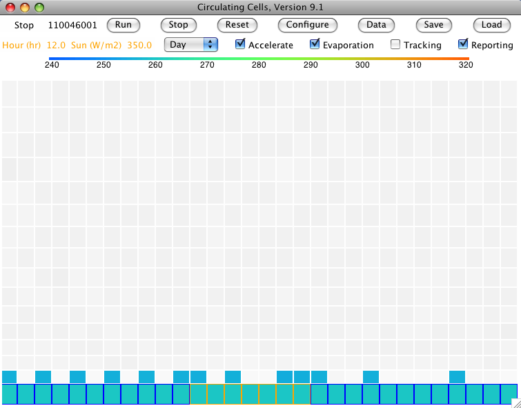
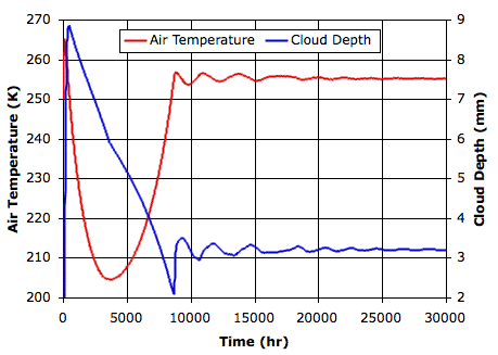
The planet warms quickly in the steady light of the Sun. After two hundred hours, the atmosphere is full of clouds and the planet starts to cool. The clouds sink towards the surface. After four thousand hours, they are thin enough that the sun starts to warm the surface. After eight thousand hours, this warming is stopped by the formation of new clouds. After a thirty thousand hours, the atmosphere settles to the steady state shown below, which you will find saved as a text array here.

The graph below plots temperature and cloud depth versus time for the first thirty thousand hours.

After thirty thousand hours, the sand and water surfaces are both at 260 K (−13°C), and the lower gas cells are at 255 K (−18°C). The average cloud depth is 3.2 mm and the average power reaching the surface is 120 W/m2.
The combination of evaporation and sinking gives rise to an equilibrium in which the clouds allow just enough heat to reach the surface so that evaporation balances the return of water to the sea in the form of sinking droplets. This balance between evaporation and sinking controls the temperature of the planet surface. In our next post, we will increase the sinking speed by a factor of a hundred and see how this affects the surface temperature. We expect the surface temperature to go up, because only then will evaporation keep up with the increased loss by sinking.
UPDATE: It turns out that our code was allowing clouds to sink only when they took part in a circulation, which resulted in them sinking roughly a hundred times slower than they should have, so our effective sinking rate in this simulation was more like 0.03 mm/s. When we correct our error, so that the clouds really do sink at 3 mm/s, the surface temperature warms by roughly 7 K. [07-JAN-12]
As we found in Simulation Time, our program checks each gas cell every one hundred iterations on average, which corresponds to every 100 s. If it takes a droplet one hundred thousand seconds to fall the height of a cell, and the droplets in the cell are evenly distributed, 0.1% of the droplets will sink out of the cell every 100 s. If the cell rests upon a surface block, these droplets will return to the surface. We now have a way for water to leave the surface, by evaporation, and a way for water to return to the surface, by sinking. If the gas cell rests upon another gas cell, the droplets enter the cell below, where they may evaporate.
In Circulating Cells Version 9.1, we specify the sinking speed of droplets at 100 kPa with sinking_speed_mps in units of meter per second. We set sinking_speed_mps to 0.003 m/s and loaded CS_0hr into our array, which is the starting condition we used in Cold Start.
The planet warms quickly in the steady light of the Sun. After two hundred hours, the atmosphere is full of clouds and the planet starts to cool. The clouds sink towards the surface. After four thousand hours, they are thin enough that the sun starts to warm the surface. After eight thousand hours, this warming is stopped by the formation of new clouds. After a thirty thousand hours, the atmosphere settles to the steady state shown below, which you will find saved as a text array here.
The graph below plots temperature and cloud depth versus time for the first thirty thousand hours.
After thirty thousand hours, the sand and water surfaces are both at 260 K (−13°C), and the lower gas cells are at 255 K (−18°C). The average cloud depth is 3.2 mm and the average power reaching the surface is 120 W/m2.
The combination of evaporation and sinking gives rise to an equilibrium in which the clouds allow just enough heat to reach the surface so that evaporation balances the return of water to the sea in the form of sinking droplets. This balance between evaporation and sinking controls the temperature of the planet surface. In our next post, we will increase the sinking speed by a factor of a hundred and see how this affects the surface temperature. We expect the surface temperature to go up, because only then will evaporation keep up with the increased loss by sinking.
UPDATE: It turns out that our code was allowing clouds to sink only when they took part in a circulation, which resulted in them sinking roughly a hundred times slower than they should have, so our effective sinking rate in this simulation was more like 0.03 mm/s. When we correct our error, so that the clouds really do sink at 3 mm/s, the surface temperature warms by roughly 7 K. [07-JAN-12]
Wednesday, November 2, 2011
Falling Droplets
In Clouds Without Rain we saw immortal clouds circulating above a frozen planet, reflecting the Sun's heat back into space. We concluded that it is rain that saves our planet from freezing. It is rain that clears the skies so that the Sun's heat can reach us.
We must implement rain in our simulation, so that water vapor has some way of returning to the surface. Let us begin by considering how fast water drops fall through air. A falling drop accelerates until air resistance matches its weight. At that point, it continues to fall but it does not accelerate. It has reached its terminal velocity. In The Terminal Velocity of Fall for Water Droplets in Stagnant Air, Gunn et al. describe their apparatus for measuring the terminal velocity of water droplets, and present their measurements in graphs and tables. (The paper, published in 1948, is an enjoyable read that you can download here.)
We can calculate the terminal velocity of rigid, spherical objects using Stokes Law. Gunn et al. show that Stokes' Law applies well to water droplets of diameter less than 100 μm (one tenth of a millimeter). You may recall that the droplets in our simulated clouds are roughly 10 μm in diameter (one hundredth of a millimeter). For the droplets are small enough, surface tension is able to maintain a spherical shape in the face of air resistance.
But for droplets larger than 100 μm, Stokes Law over-estimates the terminal velocity. Larger droplets assume flattened shapes as they fall, and they are in constant motion, so that the air resistance they encounter is far greater than it would be for a rigid sphere. When the diameter exceeds 5 mm, the motion of the drop becomes so vigorous that the drop breaks into smaller drops.
The following graph shows the Gunn et al. measurements of terminal velocity, plotted against droplet diameter. We see that the maximum terminal velocity for the largest possible water droplets is around 10 m/s. For diameters less than 0.1 mm, Gunn et al. assure us we can use the terminal velocity given by Stoke's Law, so we also plot the terminal velocity calculated from Stokes' Law.

The 10-μm droplets in our simulated clouds will fall at a mere 3 mm/s through our gas cells. Given that our cells are a few hundred meters high, it will take a day or two for a cloud to fall from one cell to the cell below. Slow as this may be, the sinking of clouds does provide a way for water to move from one cell to another, and ultimately to return to the planet surface. In our next post, we will see how sinking clouds affect the result of our Cold Start simulation.
We must implement rain in our simulation, so that water vapor has some way of returning to the surface. Let us begin by considering how fast water drops fall through air. A falling drop accelerates until air resistance matches its weight. At that point, it continues to fall but it does not accelerate. It has reached its terminal velocity. In The Terminal Velocity of Fall for Water Droplets in Stagnant Air, Gunn et al. describe their apparatus for measuring the terminal velocity of water droplets, and present their measurements in graphs and tables. (The paper, published in 1948, is an enjoyable read that you can download here.)
We can calculate the terminal velocity of rigid, spherical objects using Stokes Law. Gunn et al. show that Stokes' Law applies well to water droplets of diameter less than 100 μm (one tenth of a millimeter). You may recall that the droplets in our simulated clouds are roughly 10 μm in diameter (one hundredth of a millimeter). For the droplets are small enough, surface tension is able to maintain a spherical shape in the face of air resistance.
But for droplets larger than 100 μm, Stokes Law over-estimates the terminal velocity. Larger droplets assume flattened shapes as they fall, and they are in constant motion, so that the air resistance they encounter is far greater than it would be for a rigid sphere. When the diameter exceeds 5 mm, the motion of the drop becomes so vigorous that the drop breaks into smaller drops.
The following graph shows the Gunn et al. measurements of terminal velocity, plotted against droplet diameter. We see that the maximum terminal velocity for the largest possible water droplets is around 10 m/s. For diameters less than 0.1 mm, Gunn et al. assure us we can use the terminal velocity given by Stoke's Law, so we also plot the terminal velocity calculated from Stokes' Law.
The 10-μm droplets in our simulated clouds will fall at a mere 3 mm/s through our gas cells. Given that our cells are a few hundred meters high, it will take a day or two for a cloud to fall from one cell to the cell below. Slow as this may be, the sinking of clouds does provide a way for water to move from one cell to another, and ultimately to return to the planet surface. In our next post, we will see how sinking clouds affect the result of our Cold Start simulation.
Wednesday, October 19, 2011
Cold Start
In our previous post, we presented our simulation of clouds without rain. We started the atmospheric gas, the sandy island, and the watery sea, at a uniform 280 K (7°C). Water evaporated from the sea. The sand heated up in the sun. Hot air rose above the island and sucked moist air in from the sea. Clouds formed above the island, spread through the atmosphere, reflected the heat of the sun, and the world froze.
What if we start with a frozen world and a dry atmosphere? In our simulation of evaporation rate, no water will evaporate from a sea at 250 K (−23°C), so no clouds will form. We ran CC9, starting with the CS_0hr array, to find out what would happen. Our starting point is a uniform 250 K with no water vapor. We run with 350 W/m2 continuous heat from the Sun.
After 20 hrs, the sandy island has warmed to 276 K (3°C). At 30 hrs, the average cloud depth is 0.03 mm, which is so thin that we don't bother plotting the clouds as white cells. But at 40 hrs we start to see the first thin clouds, and the average power arriving from the Sun drops to 335 W/m2. At 50 hrs, the island reaches 283 K (10°C). From here on, it cools. At 100 hrs, the average cloud depth is 3.5 mm and only 120 W/m2 is arriving from the Sun. The sea reaches 267 K (−6°C), which is the warmest it will ever get. By 200 hrs, cloud depth is 7.2 mm and power arriving from the Sun is only 40 W/m2, as recored in CS_200hr.
We can see where the simulation is going to end up: a world kept frozen by immortal clouds. Regardless of our starting point, immortal clouds reflect the Sun's heat and cause the world to freeze.
What if we start with a frozen world and a dry atmosphere? In our simulation of evaporation rate, no water will evaporate from a sea at 250 K (−23°C), so no clouds will form. We ran CC9, starting with the CS_0hr array, to find out what would happen. Our starting point is a uniform 250 K with no water vapor. We run with 350 W/m2 continuous heat from the Sun.
After 20 hrs, the sandy island has warmed to 276 K (3°C). At 30 hrs, the average cloud depth is 0.03 mm, which is so thin that we don't bother plotting the clouds as white cells. But at 40 hrs we start to see the first thin clouds, and the average power arriving from the Sun drops to 335 W/m2. At 50 hrs, the island reaches 283 K (10°C). From here on, it cools. At 100 hrs, the average cloud depth is 3.5 mm and only 120 W/m2 is arriving from the Sun. The sea reaches 267 K (−6°C), which is the warmest it will ever get. By 200 hrs, cloud depth is 7.2 mm and power arriving from the Sun is only 40 W/m2, as recored in CS_200hr.
We can see where the simulation is going to end up: a world kept frozen by immortal clouds. Regardless of our starting point, immortal clouds reflect the Sun's heat and cause the world to freeze.
Tuesday, October 4, 2011
Clouds Without Rain
Today we present Circulating Cells Version 9 (CC9), and we use it to find out what would happen if we had clouds without rain. The simulation implements the following features of clouds.
(1) Evaporation from surface water, as in Evaporation Rate.
(2) Condensation in rising air, as in Condensation Point and Condensation Rate.
(3) Cooling and warming by latent heat of evaporation, as in Latent Heat.
(4) Reflection of incoming sunlight, as in Simulated Clouds, Part I.
The simulation does not yet implement the following features of clouds.
(5) Absorption and emission of long-wave radiation, as in Simulated Clouds, Part II.
(6) Cooling and warming by latent heat of fusion, as in Latent Heat.
(7) Rain and snow.
If we set the simulated atmosphere's transparency fraction to 0.0, we make the atmospheric gas opaque to long-wave radiation. No radiation escapes into space from the surface blocks nor from the rows of gas cells below the top row, regardless of the distribution of clouds within the atmosphere. The top row of cells, which is our simulated tropopause, does all the radiating of heat into space. Although this opaque atmosphere is not realistic, it does mask the fact that our clouds do not in themselves absorb or emit long-wave radiation, allowing us to proceed with a simulation that is at least self-consistent. Thus the copy of CC9 that you can download today has the transparency fraction set to 0.0 by default.
We ignore the warming of rising air by freezing water droplets, and the cooling of falling air by melting ice crystals. We will add ice crystals to our simulation later. For now, we trust that the error caused by our omission is not so great as to overturn the observations we make today.
By ignoring rain and snow, we are ignoring a feature of clouds that is so important to our climate that our simulation produces an entirely fantastic result. To watch the simulation in action, download CC9 and follow the instructions at the top of the code to run the program on your computer. Get the CWR_0hr array file and load it with the Load button. You will see an atmosphere at a uniform 280 K, and down at the bottom, an island of sand in a sea of water, also at 280 K. Press Run and the simulation will begin. The CC9 code runs in "Day" mode by default, with 350 W/m2 arriving continuously from the sun.
Without rain and snow, any and all moisture that enters the atmosphere at the beginning of the simulation remains in the atmosphere for as long as the simulation runs. There is no means by which moisture can return to the surface of the planet. So long as the lower atmosphere is warm enough to absorb water vapor, however, the clouds can appear and disappear. The moisture they contain can either take the form of water vapor, as it will when the surrounding gas is warm, or it can take the form of water droplets, as it will when the surrounding gas is cold.
We represent clouds in our simulation with cells that are shaded white to gray. The thinnest clouds are white and the thickest are black. A cloud with 1 mm of water is white. A cloud with 12 mm of water is black. After 30 hours, the first white clouds appear over the island, the result of moist air from the sea being heated by the island and rising towards the tropopause. When it rises, it cools, and water vapor condenses to form the first clouds.
At 40 hours, the island reaches its peak temperature of around 311 K. After that, the clouds become more numerous. They reflect the Sun's light back into space. The surface begins to cool. After 150 hrs we end up with the following display.

There is fog over the sea and part of the island. There are thick clouds up in the tropopause. The average heat arriving at the surface from the Sun has dropped from 350 W/m2 to only 50 W/m2. The following graph shows how the atmosphere cools in the first 500 hrs.

Let us refer to the combined thickness of the clouds above a surface block as is its cloud cover. In our simulation, each 3 mm of cloud cover reflects 63% of incoming sunlight. If we press the Data button, a text window opens and here we will see a line of numbers printed every hour of simulation time. The first number is the time in hours, the second is the average cloud cover in millimeters. The third number is the average sunlight power penetrating to the surface through the cloud cover in Watt per square meter. After that we have four temperatures in Kelvin: average sand temperature, average water temperature, average surface gas temperature, and average tropopause temperature. We used these printed lines to obtain the data for the plot above.
After 3000 hrs, the tropopause has dropped to 158 K (−115°C) and the surface air is at 184 K (−85°C). The average cloud cover is 25 mm. Only 0.7 W/m2 arrives at the surface. You can see this for yourself by loading CWR_3000hr into the simulation. Even at 158 K, the tropopause is still radiating 35 W/m2, which is far more than the 0.7 W/m2 reaching the planet surface. The tropopause will keep cooling until it reaches 60 K, at which point it will be radiating 0.7 W/m2. Of course, at that point, nitrogen will condense into liquid.
If clouds remained aloft in the atmosphere indefinitely, the Earth would freeze. But in reality, clouds are forever falling towards the ground. They are made of droplets and crystals that are heavier than air. Rain and snow are what stop clouds from turning the Earth into a planet of frozen seas.
(1) Evaporation from surface water, as in Evaporation Rate.
(2) Condensation in rising air, as in Condensation Point and Condensation Rate.
(3) Cooling and warming by latent heat of evaporation, as in Latent Heat.
(4) Reflection of incoming sunlight, as in Simulated Clouds, Part I.
The simulation does not yet implement the following features of clouds.
(5) Absorption and emission of long-wave radiation, as in Simulated Clouds, Part II.
(6) Cooling and warming by latent heat of fusion, as in Latent Heat.
(7) Rain and snow.
If we set the simulated atmosphere's transparency fraction to 0.0, we make the atmospheric gas opaque to long-wave radiation. No radiation escapes into space from the surface blocks nor from the rows of gas cells below the top row, regardless of the distribution of clouds within the atmosphere. The top row of cells, which is our simulated tropopause, does all the radiating of heat into space. Although this opaque atmosphere is not realistic, it does mask the fact that our clouds do not in themselves absorb or emit long-wave radiation, allowing us to proceed with a simulation that is at least self-consistent. Thus the copy of CC9 that you can download today has the transparency fraction set to 0.0 by default.
We ignore the warming of rising air by freezing water droplets, and the cooling of falling air by melting ice crystals. We will add ice crystals to our simulation later. For now, we trust that the error caused by our omission is not so great as to overturn the observations we make today.
By ignoring rain and snow, we are ignoring a feature of clouds that is so important to our climate that our simulation produces an entirely fantastic result. To watch the simulation in action, download CC9 and follow the instructions at the top of the code to run the program on your computer. Get the CWR_0hr array file and load it with the Load button. You will see an atmosphere at a uniform 280 K, and down at the bottom, an island of sand in a sea of water, also at 280 K. Press Run and the simulation will begin. The CC9 code runs in "Day" mode by default, with 350 W/m2 arriving continuously from the sun.
Without rain and snow, any and all moisture that enters the atmosphere at the beginning of the simulation remains in the atmosphere for as long as the simulation runs. There is no means by which moisture can return to the surface of the planet. So long as the lower atmosphere is warm enough to absorb water vapor, however, the clouds can appear and disappear. The moisture they contain can either take the form of water vapor, as it will when the surrounding gas is warm, or it can take the form of water droplets, as it will when the surrounding gas is cold.
We represent clouds in our simulation with cells that are shaded white to gray. The thinnest clouds are white and the thickest are black. A cloud with 1 mm of water is white. A cloud with 12 mm of water is black. After 30 hours, the first white clouds appear over the island, the result of moist air from the sea being heated by the island and rising towards the tropopause. When it rises, it cools, and water vapor condenses to form the first clouds.
At 40 hours, the island reaches its peak temperature of around 311 K. After that, the clouds become more numerous. They reflect the Sun's light back into space. The surface begins to cool. After 150 hrs we end up with the following display.
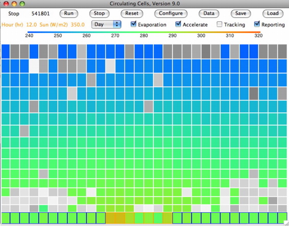
There is fog over the sea and part of the island. There are thick clouds up in the tropopause. The average heat arriving at the surface from the Sun has dropped from 350 W/m2 to only 50 W/m2. The following graph shows how the atmosphere cools in the first 500 hrs.
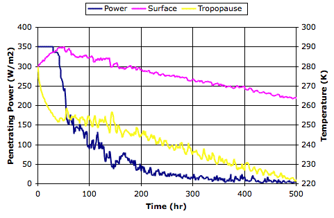
Let us refer to the combined thickness of the clouds above a surface block as is its cloud cover. In our simulation, each 3 mm of cloud cover reflects 63% of incoming sunlight. If we press the Data button, a text window opens and here we will see a line of numbers printed every hour of simulation time. The first number is the time in hours, the second is the average cloud cover in millimeters. The third number is the average sunlight power penetrating to the surface through the cloud cover in Watt per square meter. After that we have four temperatures in Kelvin: average sand temperature, average water temperature, average surface gas temperature, and average tropopause temperature. We used these printed lines to obtain the data for the plot above.
After 3000 hrs, the tropopause has dropped to 158 K (−115°C) and the surface air is at 184 K (−85°C). The average cloud cover is 25 mm. Only 0.7 W/m2 arrives at the surface. You can see this for yourself by loading CWR_3000hr into the simulation. Even at 158 K, the tropopause is still radiating 35 W/m2, which is far more than the 0.7 W/m2 reaching the planet surface. The tropopause will keep cooling until it reaches 60 K, at which point it will be radiating 0.7 W/m2. Of course, at that point, nitrogen will condense into liquid.
If clouds remained aloft in the atmosphere indefinitely, the Earth would freeze. But in reality, clouds are forever falling towards the ground. They are made of droplets and crystals that are heavier than air. Rain and snow are what stop clouds from turning the Earth into a planet of frozen seas.
Tuesday, September 27, 2011
Summary to Date
Once we were satisfied that our simulation handled convection properly, that we could relate the program iterations to the passage of time, and that all the heat entering the simulated system was accounted for by radiation from the top, we added blocks of either water or sand beneath the bottom gas cells, so as to simulate the planet surface. In Back Radiation we showed how the heat capacity and radiation produced by a semi-transparent atmosphere keeps the planet surface warm at night. In Island Inversion we see the surface of an island heating up ten times more than the surrounding ocean, while at night a layer of air a few hundred meters above the island is warmer, rather than cooler, than the air resting upon the island. Thus we see our simulation is consistent with our observations of surface cooling, including even temperature inversion.
Well-satisfied with our simulation of a dry atmosphere, we now turn to the simulation of a wet atmosphere, in which evaporation will cool the ocean and lead to the formation of clouds. To simulate cloud formation, we must have equations for the rate of evaporation from a water surface, the rate at which water vapor will condense out of rising air, the rate at which it will evaporate again in falling air, the cooling effect of evaporation upon the water surface, the warming effect of condensation upon the rising air, the amount of sunlight that will be reflected by existing clouds, and the amount of long-wave radiation that these same clouds will absorb and radiate. We obtained these relations in a series of posts Evaporation Rate to Consensation Rate. We have yet to consider the downward drift of water droplets that leads to their combining together and forming rain. But after so many posts of mathematics and empirical relations, we thought it was time to get back to the simulation, and so we will start our simulation of clouds without allowing rain, and perhaps we will see how important rain is for our climate.
We are running CC9 right now, and will present it later this week, once I have made a reasonable effort to eliminate errors from my implementation of evaporation, condensation, and reflection. The clouds are going round right now, as gray-shaded cells, and the effect is entertaining. Ultimately, you may recall, our objective is to see how a change in the transparency of the dry atmosphere affects the surface temperature of the planet, so that we can determine the effect of CO2 doubling within a system dominated by the effect of cloud formation and rain.
Well-satisfied with our simulation of a dry atmosphere, we now turn to the simulation of a wet atmosphere, in which evaporation will cool the ocean and lead to the formation of clouds. To simulate cloud formation, we must have equations for the rate of evaporation from a water surface, the rate at which water vapor will condense out of rising air, the rate at which it will evaporate again in falling air, the cooling effect of evaporation upon the water surface, the warming effect of condensation upon the rising air, the amount of sunlight that will be reflected by existing clouds, and the amount of long-wave radiation that these same clouds will absorb and radiate. We obtained these relations in a series of posts Evaporation Rate to Consensation Rate. We have yet to consider the downward drift of water droplets that leads to their combining together and forming rain. But after so many posts of mathematics and empirical relations, we thought it was time to get back to the simulation, and so we will start our simulation of clouds without allowing rain, and perhaps we will see how important rain is for our climate.
We are running CC9 right now, and will present it later this week, once I have made a reasonable effort to eliminate errors from my implementation of evaporation, condensation, and reflection. The clouds are going round right now, as gray-shaded cells, and the effect is entertaining. Ultimately, you may recall, our objective is to see how a change in the transparency of the dry atmosphere affects the surface temperature of the planet, so that we can determine the effect of CO2 doubling within a system dominated by the effect of cloud formation and rain.
Wednesday, August 10, 2011
Island Inversion
We invite you to download Circulating Cells, Version 8.4 by clicking here so that you can watch it simulate air movement above an island in the sea. Start the program and set it to Cycle mode with Q_sun set to 700 W/m2. Download this file and read it into the simulation with the Load button. You will see the an island of sand at the center of the surface blocks, surrounded by water on the left and right. The saved state of the cell corresponds to midnight, so you can start the simulation right away.
Just before dawn, at solar time 5.5 hr, you will see that the temperature of the air resting upon the sand of the island is slightly cooler than the air above. The following figure is a close-up of the air above the sand, in which ran the program with max_T set to 300 K and min_T set to 260 K in the source code so as to make the cool layer more obvious. Note that the orange-lined surface blocks are sand and the blue-lined ones are water.

Our simulation produces the inversion of atmospheric temperature that we discussed in Surface Cooling, Part IV. In that post, we proposed that the leaves of a forest would cool at night by radiation. Air in contact with the leaves would descend to the ground and drag warmer air down from above. We suggested that this process might cool the first ten to a hundred meters of air above the treetops, producing temperature inversion. Perhaps that is indeed what happens over a forest. But in our simulation, whenever the surface is cooler than the air resting upon it, we set the heat transfer by convection and conduction to zero. How, then, does inversion occur over our simulated island?
The sandy island cools by roughly 50°C to −12°C at night. At this temperature, it radiates only 260 W/m2. Of this, 130 W/m2 is absorbed by the bottom layer of the atmosphere, because we have transparency fraction set to 0.5. Meanwhile, the bottom layer of our simulated atmosphere radiates heat both night and day. At the start of the night, its temperature is around 300 K and it radiates 230 W/m2 to the sand below, which is half the heat a black body at that same temperature would radiate. By radiation alone, we see that the cells above the sand are losing 100 W/m2.
The mass of our cells is 330 kg/m2, and their heat capacity at constant pressure is 1 kJ/kg, so 100 W/m2 will cool them by roughly 1°C/hr. This is what we see during the night above our island. Inversion does not occur over the water because the water surface in our simulation has ten times the heat capacity as the sand, and so cools ten times less at night. The water continues to warm the lower atmosphere with its radiation during the night. Thus we see how back-radiation and a surface with low heat capacity work together to produce temperature inversion.
Just before dawn, at solar time 5.5 hr, you will see that the temperature of the air resting upon the sand of the island is slightly cooler than the air above. The following figure is a close-up of the air above the sand, in which ran the program with max_T set to 300 K and min_T set to 260 K in the source code so as to make the cool layer more obvious. Note that the orange-lined surface blocks are sand and the blue-lined ones are water.
Our simulation produces the inversion of atmospheric temperature that we discussed in Surface Cooling, Part IV. In that post, we proposed that the leaves of a forest would cool at night by radiation. Air in contact with the leaves would descend to the ground and drag warmer air down from above. We suggested that this process might cool the first ten to a hundred meters of air above the treetops, producing temperature inversion. Perhaps that is indeed what happens over a forest. But in our simulation, whenever the surface is cooler than the air resting upon it, we set the heat transfer by convection and conduction to zero. How, then, does inversion occur over our simulated island?
The sandy island cools by roughly 50°C to −12°C at night. At this temperature, it radiates only 260 W/m2. Of this, 130 W/m2 is absorbed by the bottom layer of the atmosphere, because we have transparency fraction set to 0.5. Meanwhile, the bottom layer of our simulated atmosphere radiates heat both night and day. At the start of the night, its temperature is around 300 K and it radiates 230 W/m2 to the sand below, which is half the heat a black body at that same temperature would radiate. By radiation alone, we see that the cells above the sand are losing 100 W/m2.
The mass of our cells is 330 kg/m2, and their heat capacity at constant pressure is 1 kJ/kg, so 100 W/m2 will cool them by roughly 1°C/hr. This is what we see during the night above our island. Inversion does not occur over the water because the water surface in our simulation has ten times the heat capacity as the sand, and so cools ten times less at night. The water continues to warm the lower atmosphere with its radiation during the night. Thus we see how back-radiation and a surface with low heat capacity work together to produce temperature inversion.
Friday, June 10, 2011
Left-Side Only
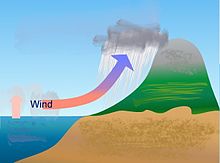
On a sunny day at the beach, the wind tends to blow towards the shore. The land warms up more than the water and warm air rises off the land. The air moving upwards sucks air sideways off the water to make the on-shore breeze. We wonder if our simulation will do something similar if we heat cells only on the left side of the array. The left-side would simulate land, and the right side would simulate water. We might see cells moving along the surface from the right, warming on the left, rising up to the top, and cooling as the move to the right again.
The figure below shows our Circulating Cells simulation program, Version 6.0, which you can download by clicking CC6. With the Left_Only box checked and Planetary Greenhouse heating, the surface cells on the left side receive twice the normal heat from the sun, while those on the right side receive none at all.

We started the simulation by loading the equilibrium state of the array with both sides receiving heat, which we have saved in PGH_Q001_M00. Following our recent discussion of enthalpy, we recognize this symmetric equilibrium state as the one in which all cells have the same enthalpy. Those at the top have more gravitational potential, but less internal heat and pressure energy, so that the sum of all three forms of energy is the same for all cells, or almost the same.
We checked the Left_Only box and increased Q_heating 0.01 K/s. You may point out that the unit of Q_heating should be Kelvin per iteration, not Kelvin per second, but we recall that one iteration corresponds to one second, so the two are equivalent. With Q_heating at 0.01 K/s, the left-side surface cells warm at 0.02 K/s and those on the right do not warm at all.
We ran the simulation for a million iterations and saved the cell array in PGH_Left_Only. The figure above shows the saved state of the cell array, after another ten thousand iterations. The temperature profile is consistent with a large-area circulation of air powered by heating on the left surface. The heated air rises to the tropopause and moves over to the right side as it radiates its heat into space. Once it has cooled, it descends to the right surface and moves along to the left.
We marked a few cells by clicking on them, and watched them go around. We invite you to do the same. The cells circulate in a clockwise direction. They rise to the tropopause on the left, but hardly ever rise to the tropopause on the right. Nevertheless, we don't see individual cells moving steadily in a clockwise direction across the width and height of the array. Often, cells rise on the extreme left and descend upon the center-left. Cells on the right rise up a little and fall again. They slowly drift to the left, but they do a lot of jumping around along the way.
When averaged over thousands of iterations, the combined movement of the cells is a large clockwise circulation, with a net movement of cells from right to left along the surface. But a simulated person standing on the center surface would not feel a steady breeze blowing from the right side. He would instead feel the wind changing every minute or two, and only by looking at the average wind speed would he be able to conclude that the net movement of air was on-shore.
Our simulation assumes that all momentum generated by circulation is dissipated as viscous heat at the end of each circulation. Thus each circulation affects only the temperature of the cells. No cell can build up momentum that encourages further circulation in the same direction.
We conclude that momentum is one of the driving forces behind the on-shore breezes. Buoyancy alone is not sufficient. If we want our simulation to produce steady winds, we must allow circulating cells to retain some of the momentum they gain during circulation, and we must allow this momentum to influence future circulations of the same cell.
The figure below shows our Circulating Cells simulation program, Version 6.0, which you can download by clicking CC6. With the Left_Only box checked and Planetary Greenhouse heating, the surface cells on the left side receive twice the normal heat from the sun, while those on the right side receive none at all.
We started the simulation by loading the equilibrium state of the array with both sides receiving heat, which we have saved in PGH_Q001_M00. Following our recent discussion of enthalpy, we recognize this symmetric equilibrium state as the one in which all cells have the same enthalpy. Those at the top have more gravitational potential, but less internal heat and pressure energy, so that the sum of all three forms of energy is the same for all cells, or almost the same.
We checked the Left_Only box and increased Q_heating 0.01 K/s. You may point out that the unit of Q_heating should be Kelvin per iteration, not Kelvin per second, but we recall that one iteration corresponds to one second, so the two are equivalent. With Q_heating at 0.01 K/s, the left-side surface cells warm at 0.02 K/s and those on the right do not warm at all.
We ran the simulation for a million iterations and saved the cell array in PGH_Left_Only. The figure above shows the saved state of the cell array, after another ten thousand iterations. The temperature profile is consistent with a large-area circulation of air powered by heating on the left surface. The heated air rises to the tropopause and moves over to the right side as it radiates its heat into space. Once it has cooled, it descends to the right surface and moves along to the left.
We marked a few cells by clicking on them, and watched them go around. We invite you to do the same. The cells circulate in a clockwise direction. They rise to the tropopause on the left, but hardly ever rise to the tropopause on the right. Nevertheless, we don't see individual cells moving steadily in a clockwise direction across the width and height of the array. Often, cells rise on the extreme left and descend upon the center-left. Cells on the right rise up a little and fall again. They slowly drift to the left, but they do a lot of jumping around along the way.
When averaged over thousands of iterations, the combined movement of the cells is a large clockwise circulation, with a net movement of cells from right to left along the surface. But a simulated person standing on the center surface would not feel a steady breeze blowing from the right side. He would instead feel the wind changing every minute or two, and only by looking at the average wind speed would he be able to conclude that the net movement of air was on-shore.
Our simulation assumes that all momentum generated by circulation is dissipated as viscous heat at the end of each circulation. Thus each circulation affects only the temperature of the cells. No cell can build up momentum that encourages further circulation in the same direction.
We conclude that momentum is one of the driving forces behind the on-shore breezes. Buoyancy alone is not sufficient. If we want our simulation to produce steady winds, we must allow circulating cells to retain some of the momentum they gain during circulation, and we must allow this momentum to influence future circulations of the same cell.
Wednesday, March 30, 2011
Surface Cooling, Part VI
We continue our study of Surface Cooling with the help of Circulating Cells, Version 5. We consider the transport of heat from a hot, sandy surface into the interior of a three-hundred meter cube of air. This three-hundred meter cube represents a single cell in the bottom row of our Rotating Greenhouse simulation. We refer to this cube as our super-cell. We are going to divide it into an array of sub-cells and heat the bottom row of sub-cells so as to induce convection within the super-cell.
We start by modifying our CC5 program. We set p_bottom to 100 kPa and p_top to 96.7 kPa. The total mass of our cell array is now 330 kg/m2, which is the mass of our super-cell. The program will create an array of sub-cells with 30 columns and 15 rows. Each sub-cell will have mass 20 kg/m2 and be 17 m high.
We set T_initial to 290 K, which is typical of a super-cell freshly-arrived at the surface our Rotating Greenhouse. We select Surface Heating, which warms the lowest sub-cells at a constant rate but allows no heat to escape from the array. According to our previous calculations, our super-cell will start to rise when it has warmed by a few degrees. Until then it will accumulate heat by convection of its own sub-cells.
When we start CC5, it calculates a value for the sub-cell impetus threshold using the procedure we describe in Impetus for Circulation. This value turns out to be 0.00003 K, a thousand times smaller than the value CC5 calculates for super-cells in our Rotating Greenhouse. As we showed in Simulation Time, each iteration of our simulation represents one second of planetary time. The heat arriving from the sun in the middle of the day can be as high as 1.4 kW/m2. Let us suppose our sandy planet surface is receiving 800 W/m2. The sub-cells have mass 20 kg/m2 and heat capacity 1 kJ/kgK. We set Q_heating to 0.04 K so that the bottom sub-cells warm at 0.04 K/s. We set our mixing fraction to 0.10. Each time a sub-cell circulates, it will exchange one tenth of its volume with its neighbors.
We reset the sub-cell array and start running. The Figure below shows the simulation after about an hour of simulated time (four thousand iterations).

We record the average temperature of our sub-cell rows and obtain the following plots.

After half an hour, the bottom row of sub-cells has warmed by 20 K and the row above has warmed by 15 K. Meanwhile, the average temperature of all the sub-cells taken together has risen by 5 K. Once it has warmed by 5 K, the super-cell is likely to rise away from the surface, so further warming will be prevented.
The sub-cells above the surface warms by ten or twenty degrees during the day. This warming provides the impetus for the local convection we proposed in our previous post. At the end of the day, sub-cell convection stops, and super-cell convection brings cool air down from above.
And so our simulation confirms the process we described in Surface Cooling, Part III. After sunset, the air temperature in a sandy desert will cool by twenty degrees within a couple of hours. Furthermore, the temperature we experience standing on the sand at mid-day will be twenty degrees warmer than the temperature of the air three hundred meters up.
We start by modifying our CC5 program. We set p_bottom to 100 kPa and p_top to 96.7 kPa. The total mass of our cell array is now 330 kg/m2, which is the mass of our super-cell. The program will create an array of sub-cells with 30 columns and 15 rows. Each sub-cell will have mass 20 kg/m2 and be 17 m high.
We set T_initial to 290 K, which is typical of a super-cell freshly-arrived at the surface our Rotating Greenhouse. We select Surface Heating, which warms the lowest sub-cells at a constant rate but allows no heat to escape from the array. According to our previous calculations, our super-cell will start to rise when it has warmed by a few degrees. Until then it will accumulate heat by convection of its own sub-cells.
When we start CC5, it calculates a value for the sub-cell impetus threshold using the procedure we describe in Impetus for Circulation. This value turns out to be 0.00003 K, a thousand times smaller than the value CC5 calculates for super-cells in our Rotating Greenhouse. As we showed in Simulation Time, each iteration of our simulation represents one second of planetary time. The heat arriving from the sun in the middle of the day can be as high as 1.4 kW/m2. Let us suppose our sandy planet surface is receiving 800 W/m2. The sub-cells have mass 20 kg/m2 and heat capacity 1 kJ/kgK. We set Q_heating to 0.04 K so that the bottom sub-cells warm at 0.04 K/s. We set our mixing fraction to 0.10. Each time a sub-cell circulates, it will exchange one tenth of its volume with its neighbors.
We reset the sub-cell array and start running. The Figure below shows the simulation after about an hour of simulated time (four thousand iterations).
We record the average temperature of our sub-cell rows and obtain the following plots.
After half an hour, the bottom row of sub-cells has warmed by 20 K and the row above has warmed by 15 K. Meanwhile, the average temperature of all the sub-cells taken together has risen by 5 K. Once it has warmed by 5 K, the super-cell is likely to rise away from the surface, so further warming will be prevented.
The sub-cells above the surface warms by ten or twenty degrees during the day. This warming provides the impetus for the local convection we proposed in our previous post. At the end of the day, sub-cell convection stops, and super-cell convection brings cool air down from above.
And so our simulation confirms the process we described in Surface Cooling, Part III. After sunset, the air temperature in a sandy desert will cool by twenty degrees within a couple of hours. Furthermore, the temperature we experience standing on the sand at mid-day will be twenty degrees warmer than the temperature of the air three hundred meters up.
Thursday, March 24, 2011
Rotating Greenhouse
The Rotating Greenhouse configuration of Circulating Cells, Version 5 simulates the cycle of day and night that results from the rotation of a Planetary Greenhouse with respect to its sun. The day_length_hr parameter gives the length of the day-night cycle in hours. In Simulation Time, we concluded that one iteration of our simulation corresponded to one second of planetary time, so one hour is 3600 iterations and one twenty-four hour day is 86400 iterations. The sun will shine upon our Rotating Greenhouse for a fraction of the day given by day_fraction. You will find both parameters in CC5's configuration array.
As in the Planetary Greenhouse, the surface is something like sand. It heats up quickly and warms the bottom cells of the atmosphere. Now that the planet is rotating, the heat from the sun increases from zero at dawn to a maximum at mid-day, and decreases to zero again at sunset. We use a sinusoidal profile for the rise in solar heating during the day. For the entire night, no heat arrives at all. In the middle of the day, heat arrives from the sun at a rate π × Q_heating. When day_fraction is one half (the days and nights are of equal length), the average rate at which the bottom cells are warmed by the sun is Q_heating. But when the day is shorter, the average warming is less than Q_heating, and when the day is longer, the average warming is greater. For now, we leave the fraction at one half.
The top cells, meanwhile, radiates heat into space just as they did for the Planetary Greenhouse. Top cells cool by Q_heating per second when they are at temperature T_balance. Their cooling rate increases as the fourth power of their temperature.
We allow the Rotating Greenhouse simulation to run. The report line gives us the time in hours instead of the iteration counter. In the top-left of the report window we see the current rate of solar heating, in units of K/hr. After many days, the cycle of day and night reaches equilibrium, and we see the following each day.

During the day, the surface cells warm as they absorb the Sun's heat. Once they warm by a few degrees, they rise, as we describe in Impetus for Circulation. The average temperature of the surface rows rises by a few degrees during the day, but not more. Our simulation does not allow surface cells to cool. And yet the average temperature of the surface row drops by a few degrees at night. When we mark a few cells near the surface, and watch them move after night falls, we see the surface cells being replaced by cooler cells from above. It is air descending from above that cools the surface row. And so our simulation confirms the mechanism for surface cooling we described in Surface Cooling, Part III.
Our simulation does not, however, show the sudden ten-degree cooling we observe standing in the desert just after the sun sets. Understanding this sudden drop was the motivation behind our Surface Cooling series of posts. Next time, we will use CC5 in its Surface Heating configuration to simulate the transport of heat within one or our large surface cells, and so obtain an estimate of how much the first twenty meters of the atmosphere will warm up during the day.
PS. You will find the array data corresponding to the start of the day with Q = 0.001 K and no cell mixing in RGH_Q001
As in the Planetary Greenhouse, the surface is something like sand. It heats up quickly and warms the bottom cells of the atmosphere. Now that the planet is rotating, the heat from the sun increases from zero at dawn to a maximum at mid-day, and decreases to zero again at sunset. We use a sinusoidal profile for the rise in solar heating during the day. For the entire night, no heat arrives at all. In the middle of the day, heat arrives from the sun at a rate π × Q_heating. When day_fraction is one half (the days and nights are of equal length), the average rate at which the bottom cells are warmed by the sun is Q_heating. But when the day is shorter, the average warming is less than Q_heating, and when the day is longer, the average warming is greater. For now, we leave the fraction at one half.
The top cells, meanwhile, radiates heat into space just as they did for the Planetary Greenhouse. Top cells cool by Q_heating per second when they are at temperature T_balance. Their cooling rate increases as the fourth power of their temperature.
We allow the Rotating Greenhouse simulation to run. The report line gives us the time in hours instead of the iteration counter. In the top-left of the report window we see the current rate of solar heating, in units of K/hr. After many days, the cycle of day and night reaches equilibrium, and we see the following each day.
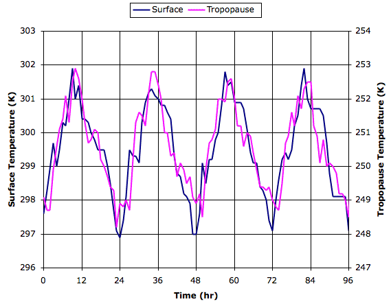
During the day, the surface cells warm as they absorb the Sun's heat. Once they warm by a few degrees, they rise, as we describe in Impetus for Circulation. The average temperature of the surface rows rises by a few degrees during the day, but not more. Our simulation does not allow surface cells to cool. And yet the average temperature of the surface row drops by a few degrees at night. When we mark a few cells near the surface, and watch them move after night falls, we see the surface cells being replaced by cooler cells from above. It is air descending from above that cools the surface row. And so our simulation confirms the mechanism for surface cooling we described in Surface Cooling, Part III.
Our simulation does not, however, show the sudden ten-degree cooling we observe standing in the desert just after the sun sets. Understanding this sudden drop was the motivation behind our Surface Cooling series of posts. Next time, we will use CC5 in its Surface Heating configuration to simulate the transport of heat within one or our large surface cells, and so obtain an estimate of how much the first twenty meters of the atmosphere will warm up during the day.
PS. You will find the array data corresponding to the start of the day with Q = 0.001 K and no cell mixing in RGH_Q001
Sunday, March 13, 2011
Summary to Date
On the side-bar, you will see a new link, Summary to Date. The new page gives a history of the posts on this site. It attempts to explain what we have achieved so far, what we are working on now, and what we hope to achieve in the future. I'll maintain the page, adding paragraphs every few months. With any luck, the page will allow newcomers to make sense of what's going on.
Wednesday, March 2, 2011
Work By Circulation
The CC3 program we presented in Planetary Greenhouse Simulation ignores the work done by cell circulation. Today we show how this omission caused the top cells to converge to a temperature 10 K lower than we expected. (Thanks to Michele for all his help in the comments.)
With Q_heating at 0.01 K, our simulation heats each cell in the bottom row by 0.01 K per iteration. With T_balance at 250 K each cell in the top row cools by 0.01 K per iteration. Our simulation assumes an ideal gas, so the heat required to warm or cool a cell by 0.01 K is always the same. At equilibrium, the heat entering must be equal to the heat leaving. We expect the top row converge to 250 K.
But the top row of CC3 converged to only 240 K. At 240 K, each top cell cools by only 0.0085 K per iteration. With circulation turned off, however, and only mixing to transport heat, the top row of CC3 did converge to exactly 250 K. We concluded that something was amiss with our circulation routine: it was making heat disappear.
In Work by Convection we showed how the expansion of warm, rising air does more work than is required to compress cool, falling air. The excess work manifests itself immediately as an upward force on the rising air. We could harness this force with a wind turbine. Otherwise the rising air will accelerate into a turbulent flow. Over time, viscous friction will transform this kinetic energy into heat. We discussed this phenomenon in Dissipation by Convection, and concluded that work by convection is what powers storms and winds.
Suppose we have a block of four cells in our simulation, at the bottom of the cell array. The lower-left cell is at 320 K while the upper-right is at 300 K. We rotate the block clockwise. The lower-left cell rises. Its pressure drops by 3.3 kPa, this being the weight per square meter of a single cell in CC3. If the cell expands adiabatically, its final temperature will be 320 K × 0.9903 = 316.90 K. Meanwhile, the upper-right cell falls. Its pressure rises by 3.3 kPa. Its final temperature will be 300 K ÷ 0.9903 = 302.94 K. One cell cooled by 3.10 K while the other warmed by 2.94 K. The two remaining cells, which do not change pressure, neither warm nor cool.
Both cells have the same mass, and the ideal gas inside has constant specific heat capacity Cp = 1.003 kJ/kg. One cell lost 3.10 kJ/kg while the other gained 2.94 kJ/kg. The difference is 160 J/kg. This 160 J/kg is the work done by the circulation. We did not account for this work in CC3. Each time a block rotated, the work by circulation disappeared.
Our CC4 program provides several new features. You can save the array temperatures to a text file, and load them also. You can track the movements and temperature of marked cells with the Tracking option. Within the code, we have greatly expanded the explanatory comments and we have simplified some of the routines and global variables to make future enhancements easier. But most important, CC4 accounts for the work done by circulation, as you can see for yourself in the circulate routine. The Viscosity option indicates whether or not we account for the dissipation of work by viscosity.
When CC4 rotates four cells, it calculate the work available just as we did above. We assume this work goes into accelerating the air within the cells and ends up dissipating as viscous friction within the four cells. The simulation adds the viscous heat to the four cells equally. The following graph shows the temperature profiles we obtained from CC4 after a million iterations for various values of mixing fraction (M) and heating rate (Q). Click on the graph for better resolution.

The top row converges to 250 K in each case. With no mixing, the bottom row is 50-K warmer than the top. With mixing fraction 0.1, the bottom is 58 K warmer than the top. With mixing fraction 0.4, it is 70 K warmer. The effect of mixing is almost exactly the same as it was for CC3. Also in the graph, you can see the profile that results when we turn off the circulation (NC) but set mixing fraction to 1.0. Heat is transported by mixing alone and the bottom is 62 K warmer than the top.
We conclude that the incorrect convergence of CC3 was indeed the result of our ignoring work by circulation. Indeed, we can obtain the CC3 results with CC4 simply by turning off CC4's viscous friction adjustment.
With Q_heating at 0.01 K, our simulation heats each cell in the bottom row by 0.01 K per iteration. With T_balance at 250 K each cell in the top row cools by 0.01 K per iteration. Our simulation assumes an ideal gas, so the heat required to warm or cool a cell by 0.01 K is always the same. At equilibrium, the heat entering must be equal to the heat leaving. We expect the top row converge to 250 K.
But the top row of CC3 converged to only 240 K. At 240 K, each top cell cools by only 0.0085 K per iteration. With circulation turned off, however, and only mixing to transport heat, the top row of CC3 did converge to exactly 250 K. We concluded that something was amiss with our circulation routine: it was making heat disappear.
In Work by Convection we showed how the expansion of warm, rising air does more work than is required to compress cool, falling air. The excess work manifests itself immediately as an upward force on the rising air. We could harness this force with a wind turbine. Otherwise the rising air will accelerate into a turbulent flow. Over time, viscous friction will transform this kinetic energy into heat. We discussed this phenomenon in Dissipation by Convection, and concluded that work by convection is what powers storms and winds.
Suppose we have a block of four cells in our simulation, at the bottom of the cell array. The lower-left cell is at 320 K while the upper-right is at 300 K. We rotate the block clockwise. The lower-left cell rises. Its pressure drops by 3.3 kPa, this being the weight per square meter of a single cell in CC3. If the cell expands adiabatically, its final temperature will be 320 K × 0.9903 = 316.90 K. Meanwhile, the upper-right cell falls. Its pressure rises by 3.3 kPa. Its final temperature will be 300 K ÷ 0.9903 = 302.94 K. One cell cooled by 3.10 K while the other warmed by 2.94 K. The two remaining cells, which do not change pressure, neither warm nor cool.
Both cells have the same mass, and the ideal gas inside has constant specific heat capacity Cp = 1.003 kJ/kg. One cell lost 3.10 kJ/kg while the other gained 2.94 kJ/kg. The difference is 160 J/kg. This 160 J/kg is the work done by the circulation. We did not account for this work in CC3. Each time a block rotated, the work by circulation disappeared.
Our CC4 program provides several new features. You can save the array temperatures to a text file, and load them also. You can track the movements and temperature of marked cells with the Tracking option. Within the code, we have greatly expanded the explanatory comments and we have simplified some of the routines and global variables to make future enhancements easier. But most important, CC4 accounts for the work done by circulation, as you can see for yourself in the circulate routine. The Viscosity option indicates whether or not we account for the dissipation of work by viscosity.
When CC4 rotates four cells, it calculate the work available just as we did above. We assume this work goes into accelerating the air within the cells and ends up dissipating as viscous friction within the four cells. The simulation adds the viscous heat to the four cells equally. The following graph shows the temperature profiles we obtained from CC4 after a million iterations for various values of mixing fraction (M) and heating rate (Q). Click on the graph for better resolution.
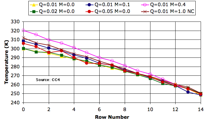
The top row converges to 250 K in each case. With no mixing, the bottom row is 50-K warmer than the top. With mixing fraction 0.1, the bottom is 58 K warmer than the top. With mixing fraction 0.4, it is 70 K warmer. The effect of mixing is almost exactly the same as it was for CC3. Also in the graph, you can see the profile that results when we turn off the circulation (NC) but set mixing fraction to 1.0. Heat is transported by mixing alone and the bottom is 62 K warmer than the top.
We conclude that the incorrect convergence of CC3 was indeed the result of our ignoring work by circulation. Indeed, we can obtain the CC3 results with CC4 simply by turning off CC4's viscous friction adjustment.
Tuesday, February 1, 2011
Mixing Cells
Our CC1 simulation allows cells to do work on one another so as to circulate by convection, but it does not allow them to pass heat to one another. The only place that heat could enter a cell was in one point along the bottom row. Today we present CC2, which allows heat to pass between cells so as to simulate mixing and conduction during atmospheric circulation. You can download the new program here.
As before, our simulation proceeds by selecting blocks of four cells at random. The simulation tests these block to see if buoyancy will cause them to rotate. In CC2, we allow heat to be exchanged between the cells of each block. We do this whether or not the cells rotate. The fraction of heat we allow to pass from each cell to each of its two neighbors is the mixing fraction. You can use CC2's new Configure button to set the mixing fraction for yourself. By default, we use 10%.
The new program provides an iteration counter, where the treatment of a block of four cells is one iteration. The display has several new buttons, as you can see below. The program starts running when you press Run. With accelerate checked, the program will update its display infrequently, so as to speed up the simulation. With the circulate and mix boxes checked, the simulation both circulates and mixes the cells. We have improved the marking of cells in this version. The marked cells have a black outline so you can see their temperature. We also increased the size of the display. Click on the following image to see the new size.

With "Point Temperature" we heat a single cell at the bottom. With "Surface Temperature" we heat all the cells along the bottom. You can set this temperature to which we heat them with the help of the Configure button.
Today we want to see how mixing affects the distribution of heat in the array with the same single-cell heating we used in our previous post. Without mixing, the cells settle down after half a million iterations to an adiabatic temperature profile, like this. With mixing the array looks pretty much the same after half a million iterations. The mixing has little effect upon the distribution of heat in the early stages of the simulation. But after 1.5 million iterations, we obtain the following array. The temperature at the top has risen from 250 K to 280 K. After two million iterations, the top of the array is at 290 K. After five million, it's above 295 K.

Half a million iterations is enough to establish an adiabatic temperature profile by convection. Five million iterations is enough to establish a uniform temperature by mixing.
We invite you to download CC2 and experiment with it yourself. For example, select surface heating to see what happens if you heat the entire bottom row of the array. Or try setting the heating temperature to 1000 K and turning off the circulation. You will see the mixing spreading heat through the array. Or run with the circulation turned on and the high heating temperature. You will see a plume of heat rising through the array.
The simulation appears to give reasonable results so far. We expected to arrive at a uniform temperature when we introduced mixing. Next time we will see what happens if we start to remove heat from the top of the array while we are inserting heat at the bottom. We wonder what type of temperature profile will evolve as heat flows up through the array.
As before, our simulation proceeds by selecting blocks of four cells at random. The simulation tests these block to see if buoyancy will cause them to rotate. In CC2, we allow heat to be exchanged between the cells of each block. We do this whether or not the cells rotate. The fraction of heat we allow to pass from each cell to each of its two neighbors is the mixing fraction. You can use CC2's new Configure button to set the mixing fraction for yourself. By default, we use 10%.
The new program provides an iteration counter, where the treatment of a block of four cells is one iteration. The display has several new buttons, as you can see below. The program starts running when you press Run. With accelerate checked, the program will update its display infrequently, so as to speed up the simulation. With the circulate and mix boxes checked, the simulation both circulates and mixes the cells. We have improved the marking of cells in this version. The marked cells have a black outline so you can see their temperature. We also increased the size of the display. Click on the following image to see the new size.
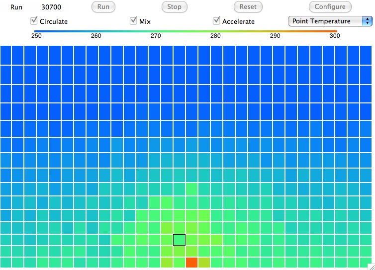
With "Point Temperature" we heat a single cell at the bottom. With "Surface Temperature" we heat all the cells along the bottom. You can set this temperature to which we heat them with the help of the Configure button.
Today we want to see how mixing affects the distribution of heat in the array with the same single-cell heating we used in our previous post. Without mixing, the cells settle down after half a million iterations to an adiabatic temperature profile, like this. With mixing the array looks pretty much the same after half a million iterations. The mixing has little effect upon the distribution of heat in the early stages of the simulation. But after 1.5 million iterations, we obtain the following array. The temperature at the top has risen from 250 K to 280 K. After two million iterations, the top of the array is at 290 K. After five million, it's above 295 K.
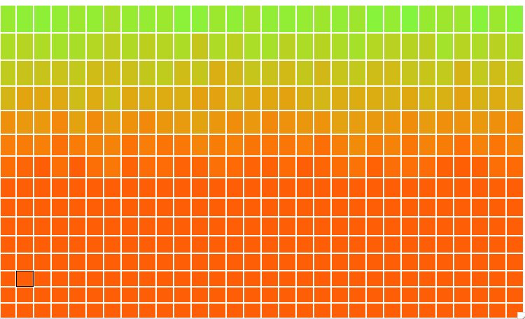
Half a million iterations is enough to establish an adiabatic temperature profile by convection. Five million iterations is enough to establish a uniform temperature by mixing.
We invite you to download CC2 and experiment with it yourself. For example, select surface heating to see what happens if you heat the entire bottom row of the array. Or try setting the heating temperature to 1000 K and turning off the circulation. You will see the mixing spreading heat through the array. Or run with the circulation turned on and the high heating temperature. You will see a plume of heat rising through the array.
The simulation appears to give reasonable results so far. We expected to arrive at a uniform temperature when we introduced mixing. Next time we will see what happens if we start to remove heat from the top of the array while we are inserting heat at the bottom. We wonder what type of temperature profile will evolve as heat flows up through the array.
Wednesday, January 26, 2011
Circulating Cells
Today we present our new simulation program, Circulating Cells, Version 1, or CC1. The following picture shows the program's display shortly after we start it up. The array of cells represents a cross-section of the atmosphere. Each cell represents an equal mass of gas. The color of the cells indicates their absolute temperature, according to the legend at the top, with the exception of the black one. The black cell is black so we can watch it circulating around.

This version of the program heats one location on the bottom row. Any cell that enters this location we heat to 300 K. If the cell enters at a higher temperature, we let it keep its higher temperature. Thus we never remove heat from our array. The hot cells are rising, and as they rise they cool down. They turn from red to green. Meanwhile, cold cells must descend to make way for the hot cells. The cells that descend warm up. They turn from blue to green. At the beginning of our simulation, all the cells are blue. They are at 250 K. If we press Reset, all the cells will return to 250 K and the simulation will start again.
In our simulation, convection occurs by rotating blocks of four cells. The program picks a block of four cells at random. It calculates how much a quarter-turn will raise or lower the block's center of gravity. If a rotation will lower the center of gravity, the program performs the rotation. Otherwise, it does not. When the program rotates a block, one cell rises, one falls, and two stay at the same height. The one that falls contracts and warms up. The one that rises expands and cools down. The two cells that move sideways do not change temperature. But they may rise when they move from the top of a cold cell to the top of a hot cell. Hot cells are taller than cold cells. In the following picture we see the distribution of heat in the atmosphere after a few minutes of running. The black cell has moved. We can turn any cell into a black cell by clicking on it with the mouse. We can turn any black cell back into a normal cell by clicking it again.

The simulation is made possible by a fundamental approximation. We arrange the cells as if the cells in each row are all at the same height, even though some may be sitting on top of columns of air that are significantly warmer or cooler than the others. Without this approximation, we cannot arrange the cells in an array, and simulation becomes several orders of magnitude more complex and time-consuming.
In CC1, there is no way for heat to pass from one cell to another. There is no conduction, no mixing, and no radiation. There is no way for heat to leave the array. After an hour of running, we end up with the following distribution of heat, all arising from the single heated location at the center of the bottom row. There is one blue cell on the bottom remaining. It moves around a bit, but so far it has resisted being drawn into the warm location.

Our program is written in TclTk. We encourage you to download the program and run it for yourself. Click here to download the program. Instructions for how to run the simulation on Linux, MacOS, and Windows are in the comments at the top of the program. Open CC_1.tcl with a text editor to read those instructions. Once the program is running, the movement of the cells is fascinating. Further comments in the program show how each routine works.
Without self-regulation by clouds we estimate that high clouds will warm the Earth by 38°C, doubling CO2 will warm the Earth by 1.5°C, and thick clouds will cool the Earth by 96°C. It is our hope that Circulating Cells will evolve into a simulation of radiation, convection, precipitation, and, ultimately, self-regulation by clouds. We will then be able to estimate the effect of doubling CO2 concentration within a self-regulating climate. That evolution may take another year or two, and maybe the task will prove too monumental for us. But I think it will be an enjoyable journey, no matter how it ends. So I hope you will accompany me.
Monday, January 17, 2011
Adiabatic Balloons
In Atmospheric Convection we described how rising air must expand and cool, while falling air must compress and warm. We used the equation for the adiabatic expansion of diatomic gases to estimate the amount by which air will cool as it rises through the atmosphere.
In a debate that took place in the comments, one of our readers claimed that a temperature difference must always exist between the bottom and the top of an atmosphere. Air is always circulating to some degree, he said, and any air that rises must cool adiabatically. He asserted that the temperature as we ascend through the atmosphere will be related to the pressure by the equation of adiabatic expansion. In Adiabatic Magic, however, we showed that our reader's claim violated the Second Law of Thermodynamics. Spontaneous adiabatic circulation of air in the atmosphere is impossible.
If spontaneous, adiabatic circulation is impossible, there must be some physical process that stops it from happening. Although we have proved that some such process must exist, we have not yet described the process. We will attempt to do so today.
Consider the following diagram. We have a column of air 5 km high, enclosed in a box. The temperature of the air is uniformly equal to 250 K. Because of the weight of the air, the pressure at the bottom is twice the pressure at the top. We have a balloon of air at the top, and another at the bottom. Each balloon is insulating and reflecting, so no heat passes in or out. Each balloon is flexible, so the pressure of the gas inside is always equal to the pressure outside.

We attach a string to the upper balloon and start to pull it down. As it descends, the air around it pushes in upon it with greater pressure so as to compress its volume. The air inside undergoes adiabatic compression. Its pressure, p, and temperature, T, are such that the product p 0.4T −1.4 remains constant.
We pull the balloon all the way down to the bottom of the column. Its pressure has doubled, so its temperature must rise from 250 K to 305 K. Our balloon has grown smaller, so the surrounding atmosphere must have expanded, and therefore cooled. But suppose our column is enormous compared to the balloon, so the cooling of the air outside the balloon is negligible. The air inside is at 305 K, and that outside remains at 250 K. The density of the air outside is 305/250 = 1.2 times greater than that of the air inside. Every kilogram of air in the balloon occupies the same volume as 1.2 kg of air outside the balloon.
By the principal of buoyancy, every kilogram of air in the balloon will experience an upward force equal to the weight of 0.2 kg of air. If we assume gravity is 10 m/s/s, we see that we must hold the balloon down with a force equal to 2 N/kg (two Newton per kilogram of air inside) or else it will rise, and it won't stop until it gets to the top again.
This buoyancy force was zero when we started pulling the balloon down, and at the end it was 2 N/kg. The average force would be close to 1 N/kg, which we apply over 5 km, so we must do roughly 5 kJ/kg of work to pull the balloon down.
Now suppose we pull the lower balloon up from the bottom at the same time. The net change in the volume of the rest of the column is is now zero, so we really can say that the outside air remains at 250 K. This other balloon, when it reaches the top of the column, will have expanded. It's pressure has halved, so its temperature must drop from 250 K to 205 K. It's density is 1.2 times greater than the air around it, so it will experience a negative buoyancy force of 2 N/kg. If we don't pull it up, it will sink all the way to the bottom again. In drawing it up, we must do 5 kJ/kg of work.
We must do 5 kJ of work to raise a single kilogram of air from the bottom to the top, and 5 kJ to lower another kilogram from the top to the bottom. Thus we see that the spontaneous circulation of air suggested by the Adiabatic Magic hypothesis is indeed impossible. It is buoyancy that stops the magic. We need a source of work to cause circulation, and no such source exists in our column of air at a uniform temperature.
One source of the necessary work is a heat engine in which we supply heat at a higher temperature to the bottom of the column and extract heat at a lower temperature from the top. Any time we have a source of heat at a higher temperature, and a place for the heat to flow to at a lower temperature, we can make a machine that does work. In the atmosphere, this machine is implemented, albeit inefficiently, by convection. We discussed work by convection earlier, but we we will return to it in future posts.
UPDATE: I originally made the column 10 km high, but Michele pointed out that I had my math wrong. The column should be 5 km high. Indeed, it turns out that the heigh of the column for which we have half the pressure at the top is a function of temperature only, which did not occur to me until I tried to duplicate Michele's calculation. See comments for details.
In a debate that took place in the comments, one of our readers claimed that a temperature difference must always exist between the bottom and the top of an atmosphere. Air is always circulating to some degree, he said, and any air that rises must cool adiabatically. He asserted that the temperature as we ascend through the atmosphere will be related to the pressure by the equation of adiabatic expansion. In Adiabatic Magic, however, we showed that our reader's claim violated the Second Law of Thermodynamics. Spontaneous adiabatic circulation of air in the atmosphere is impossible.
If spontaneous, adiabatic circulation is impossible, there must be some physical process that stops it from happening. Although we have proved that some such process must exist, we have not yet described the process. We will attempt to do so today.
Consider the following diagram. We have a column of air 5 km high, enclosed in a box. The temperature of the air is uniformly equal to 250 K. Because of the weight of the air, the pressure at the bottom is twice the pressure at the top. We have a balloon of air at the top, and another at the bottom. Each balloon is insulating and reflecting, so no heat passes in or out. Each balloon is flexible, so the pressure of the gas inside is always equal to the pressure outside.
We attach a string to the upper balloon and start to pull it down. As it descends, the air around it pushes in upon it with greater pressure so as to compress its volume. The air inside undergoes adiabatic compression. Its pressure, p, and temperature, T, are such that the product p 0.4T −1.4 remains constant.
We pull the balloon all the way down to the bottom of the column. Its pressure has doubled, so its temperature must rise from 250 K to 305 K. Our balloon has grown smaller, so the surrounding atmosphere must have expanded, and therefore cooled. But suppose our column is enormous compared to the balloon, so the cooling of the air outside the balloon is negligible. The air inside is at 305 K, and that outside remains at 250 K. The density of the air outside is 305/250 = 1.2 times greater than that of the air inside. Every kilogram of air in the balloon occupies the same volume as 1.2 kg of air outside the balloon.
By the principal of buoyancy, every kilogram of air in the balloon will experience an upward force equal to the weight of 0.2 kg of air. If we assume gravity is 10 m/s/s, we see that we must hold the balloon down with a force equal to 2 N/kg (two Newton per kilogram of air inside) or else it will rise, and it won't stop until it gets to the top again.
This buoyancy force was zero when we started pulling the balloon down, and at the end it was 2 N/kg. The average force would be close to 1 N/kg, which we apply over 5 km, so we must do roughly 5 kJ/kg of work to pull the balloon down.
Now suppose we pull the lower balloon up from the bottom at the same time. The net change in the volume of the rest of the column is is now zero, so we really can say that the outside air remains at 250 K. This other balloon, when it reaches the top of the column, will have expanded. It's pressure has halved, so its temperature must drop from 250 K to 205 K. It's density is 1.2 times greater than the air around it, so it will experience a negative buoyancy force of 2 N/kg. If we don't pull it up, it will sink all the way to the bottom again. In drawing it up, we must do 5 kJ/kg of work.
We must do 5 kJ of work to raise a single kilogram of air from the bottom to the top, and 5 kJ to lower another kilogram from the top to the bottom. Thus we see that the spontaneous circulation of air suggested by the Adiabatic Magic hypothesis is indeed impossible. It is buoyancy that stops the magic. We need a source of work to cause circulation, and no such source exists in our column of air at a uniform temperature.
One source of the necessary work is a heat engine in which we supply heat at a higher temperature to the bottom of the column and extract heat at a lower temperature from the top. Any time we have a source of heat at a higher temperature, and a place for the heat to flow to at a lower temperature, we can make a machine that does work. In the atmosphere, this machine is implemented, albeit inefficiently, by convection. We discussed work by convection earlier, but we we will return to it in future posts.
UPDATE: I originally made the column 10 km high, but Michele pointed out that I had my math wrong. The column should be 5 km high. Indeed, it turns out that the heigh of the column for which we have half the pressure at the top is a function of temperature only, which did not occur to me until I tried to duplicate Michele's calculation. See comments for details.
Saturday, January 15, 2011
Surface Cooling, Part V
If you go back and look at Surface Cooling, Part III, you will see that we have improved and abbreviated our explanation of the rapid cooling that occurs in the desert when the sun goes down. It was my father who pointed out a simple mechanism by which this cooling must occur. As we already noted, the sand will cool down quickly when the sun sets. As the day-time convection of air above the desert slows to a halt, it brings cool air down from above, and this air will not be warmed by hot sand as it was during the day. It remains cool, which causes the temperature to drop by ten or twenty degrees.
Subscribe to:
Posts (Atom)