We have described such a planet and atmosphere before, in Planetary Greenhouse. Today's CC3 program simulates the transportation of heat through such an atmosphere. You can download the program here. Running in its Planetary Greenhouse configuration, CC3 supplies heat to cells in the bottom row at a constant rate. Each bottom cell heats up by Q_heating K per iteration, regardless of its temperature. Meanwhile, a cell in the top row at temperature T_balance cools by Q_heating K per iteration. At other temperatures, the cooling rate of the upper cells increases as the fourth power of the cell temperature.
In the simulation, Q_heating represents the heat arriving from the Sun. The top cells represent the tropopause, and the heat they lose is the heat radiated by the tropopause into space. The heat radiated into space by the top cells will be equal to the heat arriving from the Sun when the temperature of all the top cells is T_balance. We start the simulation with all cells at 250 K, Q_heating = 0.01 K, and T_balance = 250 K. The top cells start to cool immediately. The lower cells start to heat up.
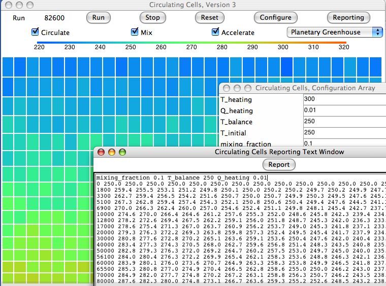
In CC3, we corrected our implementation of heat mixing in accordance with the suggestions made by Michele. You will find our new implementation in the heat routine. We added a reporting text window, as you can see in the screen shot above. You open the window with the Reporting button. The program calls report every reporting_interval iterations, or whenever you press the Report button. We instructed report to print the average temperature of the cell rows. We added a check procedure that checks for convergence of the simulation, as requested by Peter. In the comments below I'll provide some convergence code that you can paste into the check routine. In order to accommodate the planetary greenhouse temperature variations, we doubled the breadth of the color-coded temperature range. Red is now 320 K and blue is 220 K. The Configure button allows you to change the simulation parameters while the simulation is running. Be careful not to enter invalid numbers or else the program will abort with an error.
We're running the program now. It takes several hundred thousand iterations to reach equilibrium. In our next post, will present the vertical temperature profile under various conditions. We are curious to see how the temperature of the surface is affected by the amount of heat the atmosphere must transport, and by the amount of mixing we allow between cells.

Peter,
ReplyDeleteHere is some code to paste in the check routine. It stops the simulation when the bottom row gets above 280 K and at the same time the top row is within 10% of the bottom row.
set top [get_row_ave_temp $j_max]
set bottom [get_row_ave_temp 0]
if {($bottom > 280) && ([expr ($bottom-$top)/$bottom] < 0.9)} {
set cell_control "Stop"
}
Yours, Kevan
Kevan,
ReplyDeleteThanks for the quote. Just a formal point.
In the comments of program you say “When air expands adiabatically, its pressure and temperature are related by p(1-Cp/Cv)*T^-(Cp/Cv) = constant ….”
Of course there is a typo. It should be p^(1-Cp/Cv)*T^(Cp/Cv) in agreement with the same formula you wrote using the numeric exponents p^(-0.4)*T^1.4.
Michele
Dear Michele,
ReplyDeleteI have included your correction for CC4. Thank you. Do you speak Tcl? If so, can you check my implementation of the mixing? I have checked it in half a dozen ways, and it seems correct. But I'm getting a result that surprises me: a little bit of mixing increases the temperature gradient set up by circulation.
I spent an hour thinking about that last night. In the end, I think I understand how mixing slows down convection and increases gradient. But my intuition two days ago was telling me that mixing decrease the gradient. In fact, it never occurred to me that it could be otherwise.
Yours, Kevan
Kevan,
ReplyDelete** “I'm getting a result that surprises me: a little bit of mixing increases the temperature gradient set up by circulation”
There is nothing strange. In the non steady state the temperature of a cell increase both by convection and by mixing. Let’s assume we are at the first step. If the row j has been heated its temperature is Tj0 + DTc + DTm and the row j+1 is yet at T(j+1)0 = Tj0; so the gradient between the two rows is DTc + DTm greater both than DTc and DTm.
I read Tcl now for the first time. I understood the routine of mixing and it is ok for me.
Michele
Dear Michele,
ReplyDeleteI think I see what you're saying, but I'd like to understand your equations better. What are DTc and DTm?
Mixing alone will conduct heat from the surface to the tropopause. Circulation alone will transport heat. So if we combine the two, it seems reasonable to expect them to work together to decrease the required temperature gradient.
But that's not what happens in the simulation. Mixing reduces the temperature difference between neighboring cells, thus making circulation less likely. Mixing hinders circulation to such an extent that the equilibrium temperature gradient actually increases.
I see it now, and I have confirmed it with pencil and paper. But it still seems astonishing to me. Your calculation is slightly different. It would help me if I understood it better.
Yours, Kevan
Dear Kevan,
ReplyDeleteThe check routine works fine. I've added the %TempDiff between top and bottom row to the report routine. This has made it easier to see the pattern of convergence. It reaches a steady state quickly, regardless of the way the mixing_fraction or cell_mix params are used (on "Planetary Greenhouse").
Cheers,
Peter
Kevan,
ReplyDeleteYou are right; I have been too synthetic. DTc is for me DeltaTemperatureConvection, the temperature increase due to convection, and DTm is Delta Temperature Mixing, the temperature increment due to conduction.
In the non steady state, that your program simulates, a cell warms by convection&conduction and the total effect is stronger than that if one of them acts alone.
I think I have to modify my thought on the mixing.
In non steady state the unidirectional heat flow by conduction is proportional to d(dT/dz)dz and that by convection to dT/dz. That means the temperature change of a generic cell of the row ith in the array must be proportional to [T(i-1) – Ti] for the convection (assuming properly the influence of the gravity) and to [(T(i+1) – Ti) – (T(i-1) – Ti)] = [T(i+1) + T(i-1) – 2*Ti] for the conduction (mixing).
What do you think about?
Michele
Kevan,
ReplyDeleteI try to expose better my thought.
The total energy [J/kg] of the atmospheric air (having density d) is E = (Cv*T + p/d) + g*z + (u^2)/2 = Cp*T + g*z as (u^2)/2 is negligible also for the strongest storm.
Let’s consider a cell of the second row of your array. The flows of heat and mass are along z.
The convection produces at the bottom of the cell the specific entering flow rate of energy d*u*E1 [W/m^2] meanwhile at the top exit the specific flow rate d*u*E2 and the cell (having height h = z2 – z1) absorbs the specific power u*(E1 – E2)/h [W/kg] and its temperature increases at the rate dT’1/dt = u*((T1 – T2)/h – g/Cp) = u*(dT/dz – g/Cp).
By conduction at the bottom enter the specific flow rate of energy k*(T1 – T2)/h meanwhile at the top exit k*(T2 – T3)/h; the cell absorbs the specific energy k*[(T1 – T2) – (T2 – T3)]/h^2 and increases its temperature at the rate dT’’1/dt = (k/Cp)*(T1 + T3 – 2*T2).
The total increase of the cell temperature occurs at the rate dT1/dt = dT’1/dt + dT’’1/dt.
It’s very interesting to note that the steady state is reached by conduction with a linear profile of temperature (d^2T/dz^2 = 0) and by convection when the lapse rate is the adiabatic one. So an adiabatic lapse rate means that the atmosphere doesn’t warm or cool and not that it is at rest (the climatologists say that the atmosphere is stable and there isn’t convection).
Maybe anything should be changed in the climatic science!!!
Michele
Dear Peter,
ReplyDeleteI'm glad you were able to decipher the Tcl code and modify it. I am surprised to hear that the program converges "quickly". I find that it takes around half a million iterations to converge when Q_heating = 0.01, and a million to be sure of it. That's about forty minutes on my computer. Of course, I have an old computer.
Yours, Kevan
PS
ReplyDeleteOf course the increase rate of temperature is dT''/dt = (k/Cp)*(T1+T3-2*T1)/h^2
Michele
Dear Michele,
ReplyDeleteIn your comment of today, I see that the total energy of a cell is Cp*T + g*z, because the u^2/2 kinetic energy component is indeed negligible.
(By the way, you can use ρ for density with "& r h o ;" without spaces)
When you say that convection produces a "flow rate of energy" through the cell, I think you are regarding a cell location as a fixed volume, as we do when analyzing the flow in a pipe in thermodynamics, and you look at the heat flowing in the bottom boundary and out the top.
I also assume that T1 is the average temperature of the cell below, T2 is the average temperature of the cell that you study, and T3 is the temperature of the cell above.
I see your latest correction. I'm going through your equations on paper now...
I see your latest corerctio
Dear Michele,
ReplyDeleteIn the convection, we have ρ1 > ρ2. I used m as the mass flow rate in and out and continue along your lines, and arrive at the same result.
But when it comes to conduction, I see that we are assuming constant mixing fraction as we go up through the cells. But there will be very little mixing if there is no movement of air by convection, so it's not clear that my "mixing fraction" with no circulation makes any sense. Instead, we would have to consider the conductivity of air, which increases with density. Because the upper air is less dense, it will require a steeper gradient.
But I think your point is that when mixing is the largest source of heat transport, and mixing is uniform between cells of equal mass, we get a linear profile.
The question raised my our circulating cells simulation is: under what circumstances does convection take place? Does conduction encourage convection or discourage it?
In our simulation, mixing at the boundaries of cells is equivalent to conduction in your equations. I find that mixing discourages convection and so increases the temperature difference between bottom and top.
This I find astonishing. But I believe it is correct.
The simulation operates upon groups of four cells. The mixing takes place between these four cells. The convection is a rotation of the four cells. We can confirm with pencil and paper that mixing slows convection within this four-cell block. The mixing decreases the differences in temperature that drive convection.
Furthermore, going back to the Benard convection you introduced last week, we see that convection is less likely to occur when there is more diffusion of heat.
So I have the simulation, my own paper calculations, and Benard all suggesting that mixing discourages convection.
My next post will be on Mixing and Circulation, with graphs showing how big the effect of mixing is upon the equilibrium gradient. I think the result is astonishing. My worry is that there is a bug in my code.
Perhaps you could check the four-cell case yourself, to see if mixing discourages rotation. That would give me some peace of mind.
Yours, Kevan
I found a bug. In the circulate routine, this line always gives value 1.0 for the T_factor because TCL thinks R_air and Cp_air are integers, and so rounds the division to the nearest integer.
ReplyDeleteset T_factor [expr pow($p_factor,$R_air/$Cp_air)]
I have corrected this line to:
set T_factor [expr pow($p_factor,1.0*$R_air/$Cp_air)]
And now I get the correct answer for T_factor. This bug was preventing the upper cell from heating as it fell, and the rising cell from cooling as it rose. Thus it made convection more likely.
I'm running my simulations again to see how this correction affects the results.
Kevan,
ReplyDeleteI tried to expose the conservation of energy assuming the fluid was inviscid and there weren’t sources or/and sinks. Probably, my issue of language hasn’t properly given my thought when I suggested the numerical solution of the PDE that I write now formally.
ρ*δ(Cv*T+u^2/2)/δt = - ρ*u*grad(Cp*T+u^2/2) - ρ*u*g + div(k*grad(T))
that becomes for the unidirectional case along z and missing u^2/2
Cv*δT/δt = - u*(Cp*δT/δz + g) + (k/ρ)* δ^2T/δz^2
i.e.
increase rate of energy accumulation = convention contribution + conduction contribution.
When the transient vanishes, all the three terms are zero and the flow rate of energy is
by convection F’ = ρu*(Cp*T + g*z) = ρu*Cp*To W/m2
by conduction F’’ = - k*δT/δz = k*g/Cp W/m2
It’s natural that whit the same total flow rate F’ + F’’, F’ increases if F’’ decreases and vice versa.
I think the conduction can be neglected as the ratio convection/conduction is about 1.2E9 with u = 1 m/s.
Michele
Dear Michele,
ReplyDeleteVery nice Greek letters.
You have assumed that ρ is constant, which is close enough. You have assumed that k is constant, which is also close enough. For the full height of our column we would have to allow k to drop with decreasing pressure.
We have for thermal equilibrium:
(k/ρ).δ^2T/δz^2 − u.Cp.δT/δz − u.g = 0
With k=0 we have
δT/δz = −g/Cp
But this does assume that the density is constant, and so does not apply to the entire column.
With k>0 we must have δ^2T/δz^2 > 0 for a realistic solution. Thus −δT/δz must increase compared to the k=0 case, and that means δT/δz must decrease. So we will get less temperature drop from top to bottom.
This calculation gives us the result we expect: conduction reduces the temperature difference. But the calculation does not tell us where the movement of air comes from. Why is u > 0?
We have u > 0 only when the temperature difference between neighboring cells is great enough to allow them to rotate. This difference is reduced by our mixing.
I agree that conduction through air is negligible. But mixing is significant, and acts like conduction.
Yours, Kevan
PS. The bug I found did not affect the final temperatures in the simulation.
Dear Michele, In your equation let k represent the mixing, with k >0. Suppose k>0 causes u to drop. This will tend to increase δT/δz. Yours, Kevan
ReplyDeleteKevan,
ReplyDeleteThanks, I used your tip intuitively extended to the other Greek letters. That’s fine.
The density ρ can be assumed constant locally as the motion is sharply subsonic. With respect to whole column that isn’t proper because the gravity and we have to take into account the conservation of the mass stating
δρ/δt + div(ρu) = 0
and then, assuming the steady state, that ρu is constant. I think your simulation complies with the conservation of the mass as the cell height increases upward and we must consider constant within a cell all thermodynamic property of the air, which however change from a cell to another in rising.
To avoid misunderstandings is better to represent the thermal equilibrium in the form
- (ρu)*(Cp*δT/δz + g) + k*δ^2T/δz^2 = 0
In the conduction contribution k is the thermal conductivity that is never zero and, for gases at pressure > 10 kP, is not affected by the pressure being a function of the temperature alone.
Indeed, your mixing is in practice the thermal conduction that is an energy transfer at microscopic scale without macroscopic mass transfer. Rightly you don’t rotate the cells.
It seems to me that whit δ^2T/δz^2 > 0 and thus the gradient δT/δz which increases with increasing z, as the gradient is negative, its absolute value decreases. So we will get less temperature drop between the neighboring rows from bottom to top in our array and the drop of each coupe of rows will decrease over the time.
Michele
Dear Michele,
ReplyDeleteI am surprised that k, the thermal conductivity of air, remains constant with pressure. But I find that you are absolutely correct. From 10 kPa to 100 kPa at 300 K, the conductivity increases only from 0.025831 to 0.025858 W/Km. I am astonished. Thank you for educating me.
You are correct that the cells in our simulation are constant-mass, and are therefore taller as the pressure decreases.
When you say "rightly you don't rotate the cells." what do you mean? We rotate the positions of the four cells within a block to model circulation. But we do not actually rotate the cell itself so that its top surface becomes a side surface. Please explain.
Now I see that your equations should apply very well all the way up.
δT/δz = − g/Cp + (k*δ^2T/δz^2) / (ρuCp)
With k=0 we have δT/δz ≈ 0.01 K/m, which sounds about right.
I agree that with k>0, δ^2T/δz^2 has to be positive, so that δT/δz approaches zero with increasing z. This means that we should see δT/δz becoming less negative when we allow k>0.
In our simulation, mixing increases δT/δz. Is this increase realistic? If so, why is it realistic? If not, how can I fix the simulation?
Yours, Kevan
Kevan,
ReplyDeleteThanks, you’re very polite.
….."rightly you don't rotate the cells"
You use two proc. The circulating one simulate (in the transient) the convection term (ρu)*(Cp*δT/δz + g) taking into account also the gravity. The mixing one simulate (always in the transient) the conduction term k*δ^2T/δz^2 acting with the air at rest. The mixing is zero only if is δ^2T/δz^2 = 0 as k is never zero and is different from your “mixing rate” as far as I think.
I tried to solve the differential equation of the thermal equilibrium obtaining the general solution (I’m not sure about it)
T = A + Bexp(ρuCpz/k) – gz/Cp = A + Bexp(40000z) – z/100
My pc refuses to compute exp(4000) and at the top of the troposphere we would compute exp(400000000)!!!! B must be zero and we will have the well known T = T0 – z/100.
…..“mixing increases δT/δz”
I’m not able to answer and I will think about. Anyway I have a doubt: gradT produces the conduction (mixing) which produces in turn the gradT. It doesn’t sound too right. I will think about.
Michele
Dear Michele,
ReplyDeleteI get the following, after several pages of writing, and some studying my college math.
T = −gz/Cp + T(0)
− (k/ρuCp)*(T'(0)+g/Cp)*(1-exp(-zρuCp/k))
Where T(0) is T at z=0 and T'(0) is dT/dz at z=0. Thus I agree with you, and the term T'(0) must be very close to g/Cp in order for the equation to work.
I suggest we move this discussion to the comments of my next post, where I will look forward to hearing your answer.
Yours, Kevan