Carbon-14: Analytic Solution to Concentration Equations

We can describe the origin and fate of carbon-14 with a diagram or a pair of differential equations. One of the assumptions upon which we have based our reasoning so far is that one million years is more than enough for carbon-14 concentrations to reach equilibrium. Today we solve the two differential equations with a starting point of 0.0 ppt carbon-14 in the reservoir and the atmosphere. Our solution will tell us how long it takes for equilibrium concentrations to be established. For those of you who are not interested in following the derivation, we invite you to await our next post, in which we use the solution to plot graphs of carbon-14 concentration versus time.

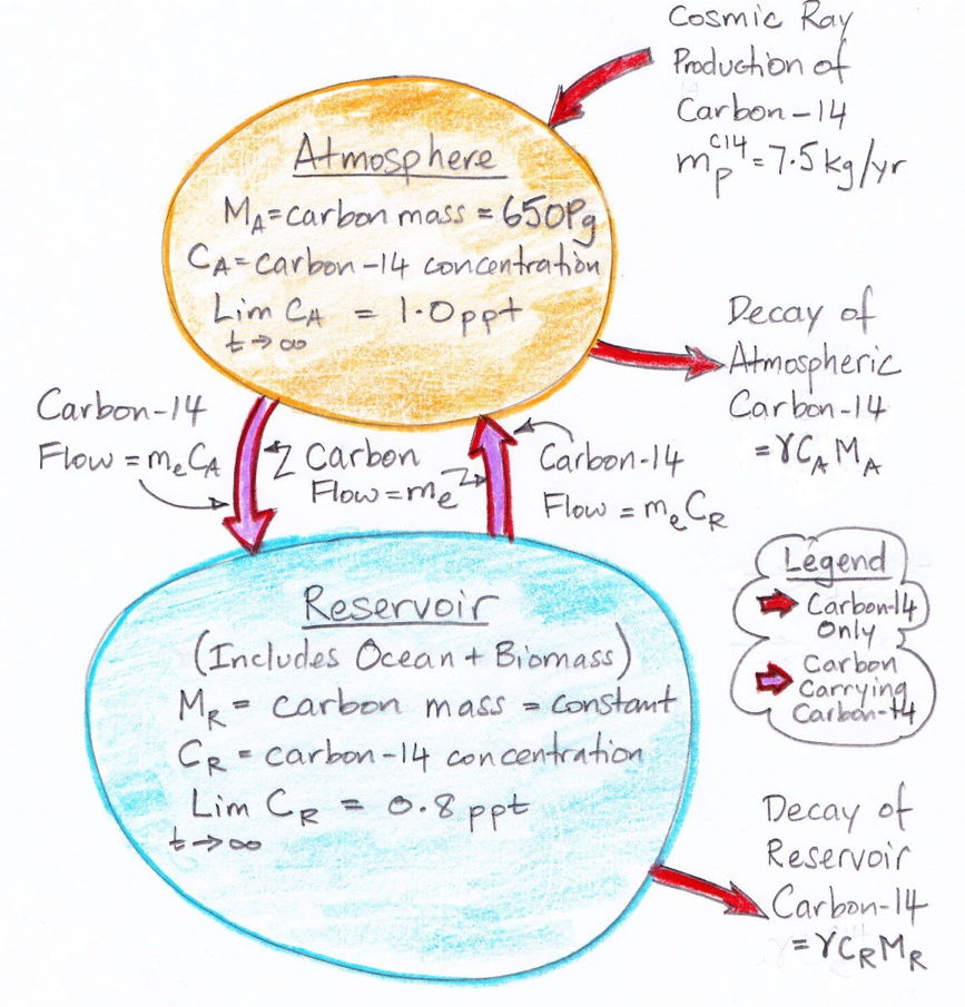
We begin by referring to our equations (1) and (2) as shown here. We re-arrange the equations so that all terms in C_A are on the left side of (1) and all terms in C_R are on the left side of (2). In doing so, we treat d/dt as if it were just another factor, which may seem odd, but it's accurate.



The only variables in these two equations are C_A, C_R, and time, t. All other parameters are constants that we have already calculated. We must eliminate C_R from the (3) so as to obtain an equation in C_A and t alone, which we can then solve. We eliminate C_R by multiplying (3) by the same factor that we observe on the left side of (4).



We do the same thing for C_R, arriving at a differential equation in only C_R and t.



At this point we pause to check the equations by considering how they behave as time approaches infinity, as shown here, and we find that they appear to behave correctly. Both equations have solutions of the same form: a constant plus two decay terms.



We insert values for m_p^C14, γ, M_A, M_R, and m_e and obtain values for all five constants in our solution. The coefficients α and β dictate how rapidly the concentration evolves with time. We have α = 0.0574 and β = 0.000122. We see that α is close to the fraction of the atmospheric carbon that is exchanged with the reservoir every year, while β is close to the decay rate of carbon-14. We have 1/α = 17 yr, which is the time constant of exchanges between the atmosphere and the reservoir, and 1/β = 8,200 yrs, which is the time constant of accumulation of carbon-14 in the reservoir. The weighting factors k₁ and k₂ are −0.2 and −0.8 respectively. Together, they add up to −1.0 ppt. The constant term is the equilibrium value of C_A, which comes out as 1.0 ppt, which is what we expect, because we chose the value of m_e and M_R to make sure that the equilibrium concentration would be 1.0 ppt. Our equation for C_A is as follows, where concentration is in ppt and time is in years.

C_A = 1.0 − 0.2 e^−t/17 − 0.8 e^−t/8200.

At t = 0, we have C_A = 0 ppt, and when t→∞, C_A→1.0 ppt, as we expect. The 17-yr decay term represents the flow of carbon-14 into the reservoir. The 8200-yr term represents the accumulation of carbon-14 in the reservoir. We obtain a similar solution for C_R.



The coefficients α' and β' are the same as α and β. But the weighting factors are different, as is the constant term. Our equation for C_R is,

C_R = 0.8 + 0.002 e^−t/17 − 0.802 e^−t/8200.

At t = 0, we have C_R = 0 ppt, and dC_R/dt = k₁α+k₂β = 0.0 ppt/yr, and d²C_R/dt² = k₁α²+k₂β² > 0, all of which we expect, and also when t→∞, we have C_R→0.8 ppt, which is one of our starting assumptions.

We are pleased to have an analytic solution for C_A and C_R. A numerical solution to the differential equations turns out to be unstable for time steps greater than ten years. We want to plot C_A and C_R over a hundred thousand years. Ten thousand steps are cumbersome in a spreadsheet. Furthermore, the analytic solution us gives more insight into the way the parameters of the carbon cycle interact to govern its behavior.