We start by modifying our CC5 program. We set p_bottom to 100 kPa and p_top to 96.7 kPa. The total mass of our cell array is now 330 kg/m2, which is the mass of our super-cell. The program will create an array of sub-cells with 30 columns and 15 rows. Each sub-cell will have mass 20 kg/m2 and be 17 m high.
We set T_initial to 290 K, which is typical of a super-cell freshly-arrived at the surface our Rotating Greenhouse. We select Surface Heating, which warms the lowest sub-cells at a constant rate but allows no heat to escape from the array. According to our previous calculations, our super-cell will start to rise when it has warmed by a few degrees. Until then it will accumulate heat by convection of its own sub-cells.
When we start CC5, it calculates a value for the sub-cell impetus threshold using the procedure we describe in Impetus for Circulation. This value turns out to be 0.00003 K, a thousand times smaller than the value CC5 calculates for super-cells in our Rotating Greenhouse. As we showed in Simulation Time, each iteration of our simulation represents one second of planetary time. The heat arriving from the sun in the middle of the day can be as high as 1.4 kW/m2. Let us suppose our sandy planet surface is receiving 800 W/m2. The sub-cells have mass 20 kg/m2 and heat capacity 1 kJ/kgK. We set Q_heating to 0.04 K so that the bottom sub-cells warm at 0.04 K/s. We set our mixing fraction to 0.10. Each time a sub-cell circulates, it will exchange one tenth of its volume with its neighbors.
We reset the sub-cell array and start running. The Figure below shows the simulation after about an hour of simulated time (four thousand iterations).
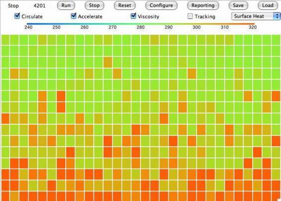
We record the average temperature of our sub-cell rows and obtain the following plots.
After half an hour, the bottom row of sub-cells has warmed by 20 K and the row above has warmed by 15 K. Meanwhile, the average temperature of all the sub-cells taken together has risen by 5 K. Once it has warmed by 5 K, the super-cell is likely to rise away from the surface, so further warming will be prevented.
The sub-cells above the surface warms by ten or twenty degrees during the day. This warming provides the impetus for the local convection we proposed in our previous post. At the end of the day, sub-cell convection stops, and super-cell convection brings cool air down from above.
And so our simulation confirms the process we described in Surface Cooling, Part III. After sunset, the air temperature in a sandy desert will cool by twenty degrees within a couple of hours. Furthermore, the temperature we experience standing on the sand at mid-day will be twenty degrees warmer than the temperature of the air three hundred meters up.

I wrote less because I was working for us.
ReplyDeleteI downloaded the free software FreeFem++ at http://www.freefem.org/ff++/ for to solve the PDE systems and I used it.
Firstly I have redone the case of “Point Temperature” solving the thermal diffusion equation
div(k(gradT)) = 0
in a domain of 30x30 km obtaining:
a) the entire domain is at 300K (the temperature of the heating point) if all the walls are adiabatic ”(heat_cond_01.png)”;
b) a radial diffusion near the point which becomes uniformly vertical near the top held at 250K whereas the others are adiabatic ”(heat_cond_02.png)”;
c) an onion diffusion if all the walls are at 250K ”(heat_cond_03.png)”.
Next I redid the case of “Surface Temperature” in the same environmental conditions with the bottom surface at 300K, obtaining:
a) the entire domain is at 300K (the temperature of the heating bottom surface) if all the walls are adiabatic ”(heat_cond_01a.png)” ;
b) a uniformly vertical diffusion in the entire domain if the top is held at 250K whereas the others are adiabatic ”(heat_cond_02a.png)”;
c) a like onion diffusion if all the remaining walls are at 250K ”(heat_cond_03a.png)”.
(follows)
Michele
Then I repeated the before steps solving the thermal convection and diffusion equation
ReplyDeleteu • grad(T) - div(k(gradT)) = 0
For the “Point Temperature” I have obtained:
a) the entire domain at 300K if all the walls are adiabatic ”(heat_cond_conv_01.png)” whatever was the vertical/horizontal velocity;
b) a radial diffusion near the point which becomes uniformly vertical near the top held at 250K whereas the others are adiabatic ”(heat_cond_conv_02_1.png)” , with a vertical velocity very little; with a velocity 5X approximately the half lower atmosphere is at 300K ”(heat_cond_conv_02_1a.png)” ; with a velocity 50X approximately the entire atmosphere is at 300K ”(heat_cond_conv_02_1b.png)” ; with a strong vertical alone and all walls at 250K one has a strong jet ”(heat_cond_conv_02_2c.png)” ;
c) a strong deformation of isothermals with a horizontal velocity very little and the top at 250K and the others adiabatic “(heat_cond_conv_02_2a.png)” ; with a velocity 50X the heat in practice doesn’t rise at all ”(heat_cond_conv_02_2a.png)” .
The case “Surface Temperature” doesn’t tell us anything of new.
That means that the convection is very important for the heat transfer through the atmosphere and we need to study the problem taking into account the Navier-Stokes equations too.
Michele
Using FreeFem++ I have solved the general problem assuming a domain 60x15 where the abscissa X=0 refers to North Pole, X=15 to Equator, X=30 to South Pole, x=45 to Equator again, X=60 to North Pole again. So we have a meridian cut of the earth. I assumed the temperature of ground is 270+40*cos(pi(1+x/15)) for the half midday meridian and 255+25cos(pi(1+(x-30)/15)) for the half midnight meridian. The top surface radiates outward al the rate 1.15e-10*T^4.
ReplyDeleteThe problem has been studied in the steady state with the follow system.
div(u) = 0 //continuity
u • grad(u) + gj + Cp*grad(T) – div(ν*grad(u)) = 0 // momentum
u • grad(CpT + gy) – div(λ*grad(T)) = 0 // total energy without KE
u • grad(k) + ε – div(μ*grad(k)) – 0.5μ*(grad(u) + grad(uT))² = 0 //kinetic turbulent energy
u • grad(ε) + a*ε² – b*div(μ*grad(ε)) – c*(grad(u) + grad(uT))² = 0 //rate of turbulent viscous energy
The results obtained after few iterations are:
a) ”temperature”;
b) ”velocities”;
c) ”kinetic turbulent energy”;
d) ”rate of turbulent viscous energy”;
What do you think about this?
Michele
Dear Michele,
ReplyDeleteThank you for sharing the results of your investigations. You have given me a lot to think about. Some of the images are quite lovely. The simulation program you downloaded appears to be quite powerful. Was it hard to install? I apologize for my website putting your comments in the SPAM folder again. I still have found no way to stop it from doing so.
Before I study the images at greater length, please check that the links are correct in the first two comments. For example, the first image you link to is a beautiful fractal-like pattern, but in your text you say it's all at 300 K.
The images in your third comment agree with your descriptions. What are μ, ν, ε and λ? What is j? I assume u is the velocity vector.
In your image of velocity, do we see the absolute value of velocity? If not, how can half of the air go up fast, while none of the air is coming down fast?
Your simulations appear to use a constant-temperature heating at the ground. In the Planetary Greenhouse simulation, we used constant-power heating, because the sandy surface heats up until it passes all its heat to the air. I will be interested to see how constant-power and constant-temperature affect your results. Of course I must take the time to understand what you have done so far before I ask you to try new things.
Yours, Kevan
The program is very simple to install and to use and its help file are very good. I had some problem with the variational calculus used by the program but I solved it quite easily.
ReplyDeleteThe links of the images are OK. The fractal images of the isothermal solutions are due to the fact that the difference between maximum and minimum are always divided into twenty parts whatever is the value of the difference. The scale aside tells the temperature varies from 300K to 300K.
The NS equation are been solved using the k – ε model for the turbulent kinetic energy (k) and its dissipation (ε), μ is the dynamic viscosity, ν the cinematic viscosity, λ the thermal conductibility, j the versor of the vertical axis and so gj is the vector of gravity acceleration.
For the velocities there are the absolute values because they are depicted as vectors.
The equation div(u) = 0 requires that the whole domain is solenoidal and so what rises must fall in any other location. The scale of the image doesn’t show well this.
The heating temperature is constant over the time. I am thinking to introduce its periodic variation.
The way used by the heat to reach the top is interesting but it is more interesting how it exit the top and the global balance of the fluxes.
Good work.
Michele
Dear Michele,
ReplyDeleteThank you for answering my questions. As you say: the links are correct when you look at the temperature scale.
Your thermal diffusion images make sense to me. I think there is a "point" left in the drawing when you heat the "surface", but the point does not do anything.
When you add a vertical velocity, how does that work? Do you allow air to flow up through the ground surface? If so, this air must acquire the temperature 300 K as it passes the bottom surface, which greatly increases the heat transported by the gas. Please explain.
In your final simulation, it appears that you are simulating an incompressible fluid, am I right? If u is velocity, your condition div(u) = 0 applies to an incompressible fluid.
Let's suppose I'm right: it's an incompressible fluid. Your velocity graph must, as you say, have as much fluid coming down as going up. But I see velocity lines going right up out of the top of the simulation. Does that mean fluid is leaving the top and entering the bottom?
I'd like to see lines that show the circulation of the fluid. In your earlier plots, you added a vertical velocity to the flow, which means gas is entering across the bottom surface. Is something similar happening in your polar velocity plot?
Yours, Kevan
The flows are activated by the gradients of the temperature.
ReplyDeleteYou are right, the fluid is assumed incompressible. Any atmospheric motion is highly subsonic and so the hypothesis is acceptable.
I have used few images making the video that I have mailed and I hope it is clear to show the air circulations.
If you download and install FreeFem++ I will post the codes used and I hope you could suggest how to improve them. I have looked for and reread my old notes of gas dynamics of the 1967, year of my degree in engineering. I did a great effort but I like it. It is challenging for a pensioner.
Michele
Dear Michele,
ReplyDeleteIf the fluid is incompressible, then it does not get thinner as it rises, so there is no dT/dz = −g/Cp drop in temperature due to convection, which explains why I see no temperature drop from bottom to top where there is no heat.
The expansion of hot gas adds another source of work to your equations. Can you allow the gas to expand as it rises?
Yours, Kevan
PS. You received your degree in 1967. I was born in 1966. Today is my birthday. I am 45. Next week my wife expects our fifth child. I hope to have some time to look at the FreeFem program, but for now I will ask you questions and look at your graphs. Yours, Kevan
ReplyDeleteMichele, Your video appears to be a Flash Player video. I'm figuring out how to play it on my MacOS computer. I am excited to see it. Yours, Kevan
ReplyDeleteKevan, my best wishes for both the circumstances. Do you think five childs are enough?
ReplyDeleteMichele
Mathematically, the “fluid dynamic incompressibility” is expressed by stating that the density ρ of a fluid parcel does not change as it moves in the flow field, i.e.,
ReplyDeleteDρ/Dt = δρ/δt + u • grad(ρ) = 0
If the time doesn’t affect the density then the local derivative δρ/δt is zero and we have a steady state. Further, if also the convection doesn’t affect the density then the convective derivative u • grad(ρ) too is zero and the fluid is “incompressible for the fluid dynamics” but it continues to be “compressible “ as for the fluid statics, i.e., according to the equation state of gases.
The continuity equation for the steady state, div(ρu) = 0, only relies each other the density and the velocity and it becomes div(u) = 0 if the density is negligibly affected by the velocity.
For the gas flow, is the Mach number that determines whether to use compressible or incompressible fluid dynamics. Roughly, the “fluid dynamic compressible” effects can be ignored at Mach numbers below about 0.3, i.e., below approximately 360 km/h at room temperature.
A little more delicate is the case of the momentum equation written in terms of accelerations as
grad(u²/2) = - g – (1/ρ)grad(p) + viscosity
because the density is strongly affected by the pressure. But if the process is adiabatic, we have
(1/ρ)grad(p) = Cp*grad(T) - (Cv*grad(T) + p*grad(V)) = Cp*grad(T)
as (Cv*grad(T) + p*grad(V)) = 0 for the adiabatics.
Thus, the momentum equation becomes
grad(u²/2) = - g – Cp*grad(T) + viscosity
totally independent from the density. Missing the viscosity we obtain along the horizontal and vertical axes
δ(u²/2)/δx = - Cp*δT/δx
δ(u²/2)/δz = - g - Cp*δT/δz
That’s, along the vertical the fluid moves uniformly if is δT/δz = - g/Cp (what a novelty!), otherwise it accelerates. Conversely, a horizontal gradient of the temperature always accelerates the fluid.
Michele
Dear Michele,
ReplyDeleteI enjoyed your equations very much. Thank you. You have produced yet another elegant derivation of the vertical lapse rate, as well as proof that any deviation from the -g/Cp lapse rate will cause the gas to slow down or speed up.
I would like to add further explanation for other readers, and show off the ∇ character:
(1/ρ)∇p = (1/ρ)∇(RT/V)
= (R/Vρ)∇T − (RT/ρV^2)∇V
For 1 kg of an ideal gas we have V=1/ρ and RT/V = p, so:
(1/ρ)∇p = R∇T − p∇V
But for an ideal gas we have R = Cp−Cv, so
(1/ρ)∇p = Cp∇T − (Cv∇T+p∇V)
For a gas, the internal energy is CvT. So Cv∇T is a vector defining the change of internal energy with position. Meanwhile, p∇V is a vector defining pressure work done with position. In adiabatic flow, the law of conservation of energy requires that the sum of the two is zero, regardless of which direction we move. The only way for this to be the case is if the two gradient vectors are equal and opposite. Thus we have
Cv∇T = −p∇V
And so we conclude that
(1/ρ)∇p = Cp∇T
In your atmospheric temperature plot at X=30 we see a 30-K drop in temperature going from surface to top of the array. What is the height of the array? It should be 3 km.
I watched your video. I saw some movement of gas within the walls of the array. I did not see an entire circulation.
Yours, Kevan
PS. I think four children is enough. But sometimes you get five even when you are happy with four. We will manage.
Dear Michele,
ReplyDeleteLooking more closely at your temperature plot, I see a 310 K drop where the ground is heated on the left, and only a 60-K drop where the ground is heated on the right. In the middle, the drop is 30 K. Such a temperature profile is not consistent with your equation:
δ(u²/2)/δz = - g - Cp*δT/δz
When there is heat to transport, the gradient will be close to −g/Cp, so we should see the same gradient on the left and right. In the center, we should see the same gradient too, or close to it, because air descending from above will be compressed and get warmed up.
Anyway: your simulation is interesting in what it tells us about convection in an incompressible fluid like water. We see that there is very little turbulent dissipation until you get to the very top of the column. And we see the fluid appears to cool as it rises. I imagine this must be due to mixing, if there is no radiation from the rising fluid.
Yours, Kevan
I have reduced Y to 10 km and also plotted the horizontal and vertical components of the velocities which are quantities with sign so it is possible to understand the sense of the eddies thermally induced. ”(velocities X90)”
ReplyDeleteI have also augmented X to 90 so the range X15 – X75 is perfectly symmetric around X45 as one can view from the new temperatures. ”(temperatures X90)”
The lapse rate is 10 K/km only without viscosity and for a uniform flow. I have plotted some lapse rates for different latitudes. At the equator the concavity of the lapse rate is positive showing that the energy of the lower atmosphere is increasing both in daytime and nighttime; for the mid latitudes the lapse rates day/night are linear; at the poles the concavity of the lapse rate is negative because the falling air is losing its energy.
”(lapse rates of temperatures)”
Michele
Dear Michele,
ReplyDeleteIn your simulation, the height of your array is significant compared to the width. But that is not the case on the Earth. So you have steady flow developing in a rotation, with hot air rising in one place and falling over the cold areas. On earth, the height of the atmosphere for convection is around 10 km, which is insignificant compared to the circumference of the Earth. The circulation you see in your simulation will start to appear in my CC6 simulation, where I hope to have a hot area and a cold area on the ground, one being sand and the other water.
Yours, Kevan