As before, our simulation proceeds by selecting blocks of four cells at random. The simulation tests these block to see if buoyancy will cause them to rotate. In CC2, we allow heat to be exchanged between the cells of each block. We do this whether or not the cells rotate. The fraction of heat we allow to pass from each cell to each of its two neighbors is the mixing fraction. You can use CC2's new Configure button to set the mixing fraction for yourself. By default, we use 10%.
The new program provides an iteration counter, where the treatment of a block of four cells is one iteration. The display has several new buttons, as you can see below. The program starts running when you press Run. With accelerate checked, the program will update its display infrequently, so as to speed up the simulation. With the circulate and mix boxes checked, the simulation both circulates and mixes the cells. We have improved the marking of cells in this version. The marked cells have a black outline so you can see their temperature. We also increased the size of the display. Click on the following image to see the new size.
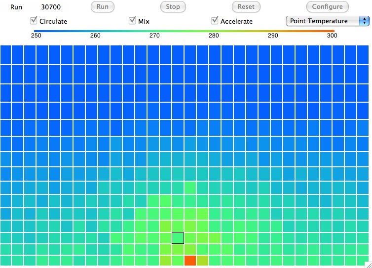
With "Point Temperature" we heat a single cell at the bottom. With "Surface Temperature" we heat all the cells along the bottom. You can set this temperature to which we heat them with the help of the Configure button.
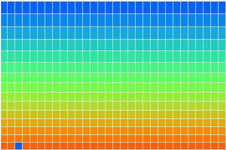
Today we want to see how mixing affects the distribution of heat in the array with the same single-cell heating we used in our previous post. Without mixing, the cells settle down after half a million iterations to an adiabatic temperature profile, like this. With mixing the array looks pretty much the same after half a million iterations. The mixing has little effect upon the distribution of heat in the early stages of the simulation. But after 1.5 million iterations, we obtain the following array. The temperature at the top has risen from 250 K to 280 K. After two million iterations, the top of the array is at 290 K. After five million, it's above 295 K.
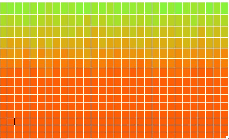
Half a million iterations is enough to establish an adiabatic temperature profile by convection. Five million iterations is enough to establish a uniform temperature by mixing.
We invite you to download CC2 and experiment with it yourself. For example, select surface heating to see what happens if you heat the entire bottom row of the array. Or try setting the heating temperature to 1000 K and turning off the circulation. You will see the mixing spreading heat through the array. Or run with the circulation turned on and the high heating temperature. You will see a plume of heat rising through the array.
The simulation appears to give reasonable results so far. We expected to arrive at a uniform temperature when we introduced mixing. Next time we will see what happens if we start to remove heat from the top of the array while we are inserting heat at the bottom. We wonder what type of temperature profile will evolve as heat flows up through the array.

Kevan,
ReplyDeleteMy congratulations for the new version of the program that is very more interactive.
The evolutions in the time of the two process (convection and mixing) are determined by the respective time scales and their comparison is possible if is used a realistic ratio of them. It is natural that the result of the mixing is gotten in a time 10X that of the convection if you assume the convection is 10X faster than the mixing.
I am asking myself and I also ask you what can be the realistic values of these parameters. I don't find answers and I hope that you would have some.
Michele
Dear Michele,
ReplyDeleteYou are very kind, thank you. I have not come to a conclusion about the mixing fraction and the convection.
From what I have read about convection, and from talking to my father who has some experience in chemical engineering, the air flow in convection is turbulent and chaotic. That's why I thought it would be okay to model convection as small circulations of four cells. And indeed I'm satisfied with the results. We see hot cells climbing up to the top, simply by the action of repeated four-cell rotations.
Now that it comes to mixing, I picked 10% mixing because I figured that was a nice fraction, and more realistic than 1%. The result is the 10X you pointed out.
I suggest we continue to the heat flow simulation, where we have heat leaving the top, and see what kind of profile we get. If it's very different from what we observe on Earth, we could consider changing the mixing fraction and seeing if that improves the match.
Of course, I would greatly appreciate your sharing any ideas you have on the subject.
Yours, Kevan
Kevan,
ReplyDeleteI slept on it and this morning I have probably a reasonable answer.
The fluid dynamics of natural convection (approximation of Rayleigh-Bénard) is based on the dimensionless Rayleigh number (Ra), that may also be viewed as the ratio of heat convection and heat diffusion. When Ra is below the critical value for that fluid, heat transfer is mostly in the form of diffusion; when it exceeds the critical value, heat transfer is above all in the form of convection.
In other words the convection rolls develop when Ra exceeds a critical value Rc , which is at least 27*pi^4/4 = 658. That means the mixing ratio would be at latest 0,0015 and the thermal diffusion is thoroughly negligible in the presence of thermal convection.
You say “the air flow in convection is turbulent and chaotic”. The natural convection air flow starts with zero velocity when the acting force exceeds the viscous resistance due to variation of form of the cell, then increase its velocity in laminar conditions (there are be added the Newton’s viscous forces) and only when Reynolds number exceeds its critical value the air flow becomes turbulent. For the natural convection the transition from laminar to turbulent flow can be also referred to Ra. If Ra < 10^9 then the flow is always laminar. If Ra > 10^10 then the flow is always turbulent. If 10^9 < Ra < 10^10 then we are in transition region and the previous flow is maintained.
I think you would use a mixing ratio of at least 10^-10 if you want simulate a turbulent natural convection. But in this case the thermal diffusion is wholly insignificant.
Michele
Dear Michele,
ReplyDeleteThat's fascinating. I did some reading on Benard cells and the Ra parameter you describe. I think you have indeed found a reasonable answer.
First off, my use of the word "turbulent" is incorrect when applied to atmospheric convection. The cells in our simulation are around 300 m high at the bottom and have mass 333 kg/m2. If we imagine them being 300 m wide as well, we have a cell so large that if it it rises by 300 m to take the place of the cell above, there is no reason to suppose that the air movement inside the cell will be turbulent.
Our simulation models convection as a sum of randomly-selected four-cell rotations. This represents the idea that convection in a free atmosphere will favor small circulations over large, tall circulations.
Now here comes Benard convection, which suggests that convection can look like my drawing of sustained, alternating cells over the desert.
I'm going to calculate the Ra for some atmospheric columns. It seems to me that there is an error of sign in the Wikipedia formula, so I'll have to check that first.
Yours, Kevan
Dear Michele,
ReplyDeleteThere is a fine picture of Benard convection cells at Wikepedia. I'm going to change the sign of their formula for Ra. I think the correct formula is:
Ra = gΒ(Tb - Tt)L^3/να
where g is gravity (10 m/s^2), Β is thermal expansion coefficient (0.003 for air at 300 K), Tb and Tt are bottom and top temperatures for the convection cycle, L is the height, ν is kinematic viscosity (18×10^-6 Pa-s), and α is thermal diffusivity (22×10^-6 m2/s).
So far as I understand, the "diffusivity" is not the mixing fraction, but the ratio of the thermal conductivity to the volumetric heat capacity.
Suppose we have L = 6000 m and (Tb-Tt) = 50 K, which is the case for the entire height of our cell array at the start of our simulation.
Ra = 10 * 0.003 * 50 * 6000^3 / (18 * 22) &asump; 10^9
According to your numbers, a column this high will be on the verge of turbulence. If it gets stirred up in any way, the Benard cell will collaps. Given that we have prevailing winds in the atmosphere, I think it likely that the limit for Benard cells is far less than 10^9, say 10^8 or 10^7.
But if we look at at L = 600 m and (Tb-Tt) = 10 K we have:
Ra = 10 * 0.003 * 10 * 600^3 / (18 * 22) ≈ 10^4
This value is so low, we can be confident that our four-cell convection cycles will indeed be laminar. The cells will slide past one another without turbulence to encourage mixing. If we have two bodies of air sliding past one another, I imagine that the mixing must penetrate at least at 0.1 m/s or more. If one body rises 300 m at 1 m/s, mixing will penetrate 30 m as it rises.
I think that 10% mixing in our four-cell blocks is a good start. I don't think 100% is reasonable, and 1% would be consistent with far larger cells. And I am content for the moment with the four-cell convection because the ten-cell convection appears delicate.
What do you think of that? Have I done my math right?
Yours, Kevan
Dear Kevan,
ReplyDeleteTo make it easier to note the different effect when varying the parameters, would it be possible to introduce the option to stop the run when a certain condition has been met, so you can note how many cycles it took for the effect to be reached.
E.g.
If the bottom_row_average_temp > a ; stop when top_row_average_temp is within b% of bottom_row_average_temp.
Cheers,
Peter
Kevan,
ReplyDeleteYou are right, there is a typo in the Wikepedia formula.
I explain my thought about the Ra number. It is the ratio of effects produced by thermal buoyancy to those of thermal diffusivity and so it also represents the ratio of diffusion time scale to convection time scale. What you name “mixing ratio” seems to correspond to 1/Ra as it affect in a similar manner the number of cycles needed to obtain the respective results in the numeric simulation by the circulation and the diffusion.
I ran CC_2.tcl setting the mixing ratio at one and it doesn’t converge but continuously changes between 250 and 300 K. I suggest to apply the mixing ratio to difference between the mean temperature of the four cells and that of each cell. I will try myself to modify the code.
Michele
Kevan,
ReplyDeleteI have to rectify me.
The temperatures have stable convergence only for mr <= 0.5.
They unstably converge for 0.5 1.
See here.
Michele
Dear Peter,
ReplyDeleteI can add that termination rule to the while loop that runs the simulation. But your question brings up the more general issue of users specifying their own termination criteria. I have been thinking about how best to give the user control over the termination.
One way that's easy for me is to have the while loop call a termination routine defined by the user. But that requires the user to learn Tcl.
I propose that I add to the code an averaging routine for rows, and then give you some sample code that implements your criterion. You would paste the sample code into an area marked in the code by a comment.
With the sample code as a starting point, you could change your numbers a and b to suit yourself.
How does that sound?
Yours, Kevan
Dear Michele,
ReplyDeleteYes, the mixing will not converge for mr > 0.5. My implementation assumed the mixing ratio is small. At mr = 1.0, we have cells exchanging all their heat with their neighbors, which does not make any sense. If one cell was very hot, it would make both its neighbors very hot and get cool itself, thus generating heat out of nothing.
Even with mr = 0.1 we see that it is indeed possible for heat to be generated and destroyed by the simulation because the implementation does not obey the First Law of Thermodynamics.
So I think you have made your point: the mixing ratio needs to be implemented differently. Furthermore, I think your average of four blocks idea is the best we can do.
Here is what i understand by your idea. At mr = 1.0, we combine the heat from all four cells and divide it equally between them. We leave each cell with its pre-existing pressure energy and potential energy. All cells end up at some temperature Ta = (T1 + T2 + T3 + T4) / 4. At mr = 0.0, we have no exchange of heat. Each cell has its own temperature Tn.
For intermediate values, we let the cells have temperature Tn + mr * (Ta - Tn). This calculation keeps the sum of the temperatures constant. Because all the cells have equal mass, and because the heat capacity of air at constant volume changes very little with temperature, I believe this means that the total heat is constant too.
What do you think of that?
Yours, Kevan
Dear Michele,
ReplyDeleteOh, I missed your link to your graphs until just this moment. Very nice. It's amazing how the discrete simulation gives such beautiful sine waves, including the damped harmonic behavior.
Yours, Kevan
Dear Kevan,
ReplyDeleteThat sounds fine.
Cheers,
Peter
Kevan,
ReplyDeleteI agree with you. The thermal mixing is a isoenergetic process as inside the cells there isn’t a source or a sink for heat. So there must be Sum(Ci*Ti) = Sum(Ci0*Ti0) during the mixing and the temperature of cells will tend to Tf = Sum(Ci*Ti)/Sum(Ci). In our case is Ci = const and so Sum(Ti) = Sum(Ti0) and Tf = Sum(Ti)/4.
I think that mr should be the % of the remaining mixing which occurs in one step of the numeric simulation and the final result will be exponentially reached with a geometric series.
Michele