Simulated Planet Surface

Our Circulating Cells Version 8.3 simulates the planet surface with a row of blocks. You can download the latest code here. These blocks can be sand or water. If they are sand, they have low heat capacity and warm up quickly in the Sun's light. If they are water, they have high heat capacity and warm up slowly. By clicking upon one of the blocks, we change it from one type to the other.

In the long run, we will implement evaporation from the water blocks, but for now we concentrate upon the heat exchange between the surface and the atmosphere. In previous versions of our program, we allowed sunlight to pass directly into the surface gas cells. Now we allow sunlight to pass all the way through the entire atmosphere to be absorbed at a solid or liquid surface. Real water reflects 4% of short-wave radiation, and sand reflects something like 10%, but our simulated water and sand absorbs all short-wave radiation.

Both sand and water are near-perfect emitters of long-wave radiation, so we allow our surface blocks to radiate heat according to Stefan's Law. We also allow heat to leave the surface blocks by convection. We determine the convection heat loss by multiplying the temperature difference between the surface and the gas by a convection coefficient. This heat leaves the surface block and enters the gas cell above.

As we described in our previous post, our simulated atmosphere is partially-transparent, to an extent specified by the transparency fraction, τ. The gas above a surface block absorbs a fraction 1−τ of the block's radiation, and the remainder passes out into space. We add the absorbed heat to the gas cell above the surface block.

Now we come to a component in the heat exchange between the atmosphere and the surface that we have not simulated or calculated before. The atmosphere itself will radiate heat downwards towards the surface, and the surface, being a perfect absorber of such radiation, will absorb all of it. The heat radiated downward by the atmosphere is often called back-radiation or downward long-wave radiation. To calculate the back-radiation, we use the same equation we applied to the tropopause in our previous post. When the transparency fraction is 0.5, the gas radiates half as much heat as a black body at the same temperature.

We ran our simulation with Day heating of 350 W/m², all surface blocks made of sand, convection coefficient 20 W/m²K, and transparency fraction 0.50. The following figure shows the equilibrium state of the array. The surface blocks are color-coded for temperature in the same way as the gas cells, but they have an orange border to mark them as sand. A water cell has a blue border. You will find the equilibrium state of the array saved as a text file here.



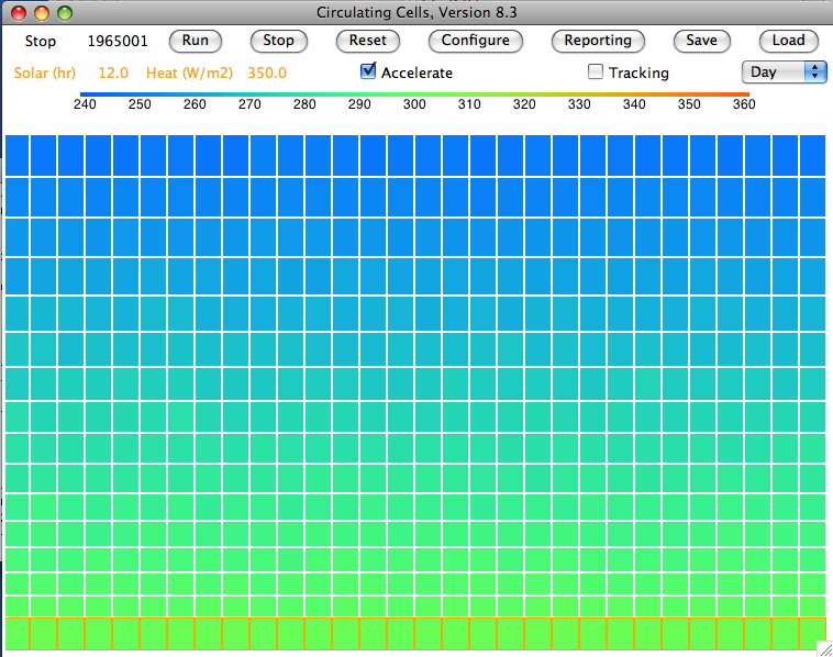
As in our previous simulations, the temperature drop from the surface gas cells to the tropopause gas cells is very close to 50 K. The sandy surface settles to 303.0 K, at which temperature it radiates 480 W/m². Of this, 240 W/m² passes directly into space and 240 W/m² is absorbed by the gas above. The tropopause settles to 249.0 K and radiates 110 W/m² into space. The total radiation into space is 350 W/m², which is the amount that is arriving from the sun, so our planet is in thermal equilibrium.

The 110 W/m² radiated by the tropopause must pass up through the atmosphere by convection. The surface gas is at an average temperature of 298.5 K, radiating 226 W/m² back to the surface. Thus a net 14 W/m² passes from the surface to the atmosphere by radiation. The remaining 96 W/m² passes into the atmosphere by convection at the surface. The surface is on average 4.5 K warmer than the gas, for which we expect only 90 W/m² to flow by convection. But the gas cells warm by roughly 8 K while they sit upon the sand. When they first arrive from above, they are almost 10 K cooler, and 200 W/m² flows into them by convection. Just before they rise up, they are only 2 K cooler, at which point only 40 W/m² flows into them. When we get the program to print out the convection rate, we obtain an average of 96 W/m², so all the heat from the Sun is accounted for.

We note that almost all the heat flowing from the surface to the atmosphere is carried by convection. The heat radiated by the surface and absorbed by the atmosphere is nearly balanced by the radiation returned by this same atmosphere. The difference is only 14 W/m², compared to 96 W/m² passing into the gas by convection. In our next post, we will simulate night and day over a sandy desert and see if we come up with reasonable variations in temperature at the sandy surface, the air above the surface, and the air high up in the tropopause.

Simulated CO2 Doubling

In Planetary Greenhouse we considered an atmosphere transparent to some long-wave radiation and opaque to others. In Circulating Cells Version 8.2, which you can download here, we simulate such an atmosphere with the new transparency fraction parameter.

For the moment, we ignore the temperature difference that must exist between the planet surface and the lower atmosphere (see Surface Cooling, Part VI). We assume that the solid or liquid surface beneath one of the bottom gas cells will be at the same temperature as the gas itself. Ever since our Earth Radiator post, we have assumed that the surface of a planet is a black body radiator. If a bottom cell is at 300 K, the surface below will be at 300 K also, and by Stefan's Law it will radiate 460 W/m². At 303 K, the radiated power increases to 480 W/m². Black-body radiation increases as the fourth power of the temperature, so a 1% increase in temperature causes a 4% increase in radiated power.

The absorption spectrum of the Earth's atmospheric layers varies in a complex and dramatic way with wavelength, as you can see here. What made our Total Escaping Power calculation so complicated was that we had to deal with the partial absorption of some wavelengths by each atmospheric layer, and therefore the partial emission of these same wavelengths by the same atmospheric layers. We want to avoid the complexity of partial absorption at a given wavelength, so we assume that the gas in our CC8 simulation has a spectrum that vacillates between perfect transparency to perfect opacity, and does so every fraction of a micron on the wavelength scale. As a result of this vacillation, a gas cell will absorb none of the radiation at a particular wavelength, or all of it. When we look at the fraction of black-body radiation that passes through a cell, this fraction is a constant property of the cell, regardless of its temperature or pressure. We call it the transparency fraction in the CC8 program, and here we will call it τ.

By the principle of radiative symmetry, each gas cells will radiate heat at the same wavelengths it absorbs. But because all the cells around it have the same absorption spectrum, none of the heat radiated by a cell will escape into space, except for the heat radiated by the cells in the top row, which we call our tropopause. These cells radiate directly into space. The power they radiate is the power that a black body would radiate, multiplied by 1−τ.

The incoming heat from the Sun, meanwhile, passes straight through our atmosphere, because we assume that the gas is perfectly transparent to short-wave radiation. The Sun's heat warms the planet surface, which for the moment we assume is something like sand. The sand heats up rapidly until it is losing heat by radiation and convection at the same rate it is gaining heat by absorption of the Sun's light. Some heat it radiates directly into space. The rest passes into the lower atmosphere and must be transported up to the tropopause by convection, where it is radiated into space.

Bottom Gas Cell Temperature = T_B
Planet Surface Temperature = T_S = T_B
Stefan's Constant = σ = 5.7 × 10⁻⁸ W/m²/K⁴
Emitted Surface Radiation = σ(T_S)⁴
Escaping Surface Radiation = τσ(T_S)⁴
Top Gas Cell Temperature = T_T
Emitted Tropopause Radiation = σ(1-τ)(T_T)⁴

We set τ=0.50 and ran CC8 with Day heating and the Sun's power set to 350 W/m². After ten million iterations we are confident that we have reached equilibrium, and we obtain this array. The average temperature of the bottom cells is 301.1 K (28°C) and of the top cells is 252.1 K (−21°C). The heat radiated by the surface is 468.5 W/m², of which 234.2 W/m² escapes directly into space. That leaves 115.7 W/m² of the Sun's heat to be transported up through the atmosphere. The heat radiated by the tropopause is 115.1 W/m², leaving 0.7 W/m² unaccounted for, which is well within the range of our rounding errors and the random fluctuations in our cell temperatures.

In our previous post, we ran our simulation for an opaque atmosphere, which corresponds to τ=0.00, and the surface temperature rose to 355 K (59°C). We see that τ=0.50 allows the surface to cool by 31°C to 28°C. In With 660 ppm CO2, we showed that doubling the CO2 concentration in the Earth's atmosphere will cause a 2% drop in the total escaping power. So now we set τ=0.49, so as to cause a 2% drop in the power escaping directly from our simulated planet surface into space. We arrive at a this array, in which the surface has warmed by 0.9°C to 302.0 K and the tropopause has warmed by 0.4°C to 252.5 K.

As a check, we run with τ=1.00, in which case the atmosphere is perfectly transparent and the surface radiates all its heat directly into space. The surface cools to 280 K (7°C). The atmosphere assumes the dry adiabatic lapse profile. But now we turn on the cell mixing by setting the mixing fraction to 0.2, and after a few hundred thousand iterations we see the entire atmosphere warm up to 280 K. This is the warm atmosphere we described in our original Greenhouse Effect post and again in Adiabatic Magic. When the atmosphere is not transporting heat to the tropopause, there is no greenhouse effect, and the atmosphere mixes until it arrives at a uniform temperature equal to the surface temperature.

We see that CC8 can simulate the effect of changing the concentration of a greenhouse gas like CO2, simply by making small changes to its transparency fraction. Once we have included evaporation, clouds, and rain into our simulation, we will be able to estimate the effect of changes in CO2 upon the average temperature of our planet surface.

Black-Body Tropopause

Our CC7 program provides six different ways to heat the atmospheric cell array. In CC8, we eliminate most of these and replace them with only three: Day, Night, and Cycle. The others were useful in checking the performance of the simulation, but are no longer necessary. Because we now have a good understanding of the relationship between simulation time, impetus for circulation, and program iterations, we are now able to express the Sun's heat in W/m² instead of the less realistic K/iteration of our earlier programs. We represent the incoming solar power with Q_sun instead of the previous Q_heating. Furthermore, we can use Stefan's Law directly upon the top cells, as if they were black and the gas above them were transparent. Our program now contains a value for Stefan's Constant, which we set to 5.7×10⁻⁸.

For our convenience, we display the time of day in hours in the main window. Time 12.0 hr is noon, when the Sun is certain to shine, and midnight is 0.0 hr. We display the current solar power in W/m². Previously, we applied a sinusoidal variation in the Sun's power during the day, but now we simply turn the Sun's power on to Q_sun during daylight hours, and to zero during the night. As before, however, the Sun will shine for a fraction of the day given by day_fraction.

We run the program with Day heating and the Sun's power set to 350 W/m². We have ke_fraction at 0.0 and we un-check left_only. Our cells have mass 333 kg/m². Their specific heat capacity at constant pressure is 1 kJ/K. Thus the lower cells warm up at 0.001 K/s, which matches our previous Q_heating of 0.001 K/iteration. We allow the array to reach equilibrium, which takes a long time: five million iterations, or one hours on our lap-top. You will find the equilibrium state in Day_1.txt. You can load it into CC8 with the Load button. At equilibrium, the top row's average temperature is 280.0 K. Applying Stefan's Law, the top cells should radiate 350 W/m², which is what we expect, since that's what we are putting in. The surface cell average temperature is 335.4 K, giving us the 55-K drop from the surface to the tropopause. This drop is consistent with our previous results.

We run the program with Q_sun set to 700 W/m² and Cycle heating to simulate day and night. We have day_fraction set to 0.5. After a million iterations we see the temperature of the bottom and top rows varying by a few degrees during night and day, as we did in Rotating Greenhouse.

The equilibrium surface temperature of 59°C (335 K) is much hotter than the surface of the Earth (around 14°C), even though 350 W/m² is the average power of the Sun. The Earth is cooler because its surface and lower atmospheric layers are able to radiate almost half their heat directly into space, assuming there is no cloud cover (see Total Escaping Power and subsequent posts).

Our next step is to allow the surface cells to radiate directly into space, and we will see how the surface cools down as a result. We must implement the surface and tropopause radiation before we can model the effect of clouds.

Cells with Momentum

We invite you to download Circulating Cells 7 by clicking here. Each cell now has vertical and horizontal kinetic energy in the manner we described in Cell Kinetic Energy.

The preservation of momentum after a circulation is controlled by the ke_fraction parameter. By default, this parameter is 0.0, and the simulation will run exactly as before, with the entire impetus for convection being transformed into viscous friction. But with ke_fraction set to 0.9, 90% of the impetus for convection will turn into kinetic energy.

In version 7.0, we have have no graphical illustration of the cell kinetic energy. Perhaps we can use short lines within the cells to indicate momentum in the future. But we can always can stop the simulation and save the array to a text file. The text file tells us the state of each cell. Text files written by 7.0 have a new format, as shown below. But please note that 7.0 can read in text files written by previous versions of the simulation.

row column marking temperature vertical_ke horizontal_ke

In the future, we will add moisture content and cloud concentration to this list of properties. For now, the cells remain dry. The kinetic energy is in units of J/kg, so if we want to know how fast the cell is moving, we take the absolute value of the kinetic energy, double it, and take the square root. If the energy is 32 J/kg, the speed is 8 m/s. The direction is given by the sign of the kinetic energy: positive is up or right.

We have been playing around with CC7, using the Left-Only and Planetary Greenhouse. We set ke_fraction to 0.9 and looked to see if a breeze developed along the lowest row of cells, from right to left. After several hundred thousand iterations, we saved the array to disk and find that all the cells along the bottom row are moving to the left, while all the cells along the top row are moving to the right. By marking cells, we can observe these movements as the simulation runs. We don't see a simple clockwise rotation: there is a lot of random movement on top of the rotation. In the middle rows, the cell movements are as random as they were in our original Left-Side Only simulation with no accounting for momentum. But along the surface and along the tropopause, we appear to have the prevailing breeze we were looking for.

What we have yet to determine is what value of ke_fraction is required to establish a steady breeze, and what fraction is realistic. We invite you to download the code and play with it yourself. We hope the implementation of kinetic energy is correct, but if not we hope you will point out any problems.

UPDATE: There is a flaw in the way we combine cell kinetic energy with impetus for circulation. When we subtract the kinetic energy of a cell from the impetus, this kinetic energy ends up disappearing from the array. We observed a similar program-induced loss of energy in Work by Circulation. Given that the effect of preserving cell momentum was not dramatic, we resolve to remove the kinetic energy calculation from our code, so that ke_fraction will remain zero.

Cell Kinetic Energy

When a block of four cells rotates within our Circulating Cells simulation, the rotation does work, and we call this work the impetus for circulation. We express the impetus for circulation in units of energy per kilogram of gas in the four cells (J/kg). In our CC6 program, we take the impetus for circulation and add it back into the gas as heat. Our assumption is that the impetus is first used to accelerate the gas, and so turns into kinetic energy, but later is dissipated as viscous friction. At the end of our circulation, the gas is once again at rest.

But clearly the gas will not be at rest at the end of a circulation. Once it starts moving, it will tend to continue moving. In our previous post we showed that the cells coming to stop means that our simulation will never allow convection to produce a steady breeze. We would like our simulation to allow a cell to retain some of its kinetic energy after the circulation is complete, and thus allow this kinetic energy to influence subsequent movements of the same cell.

We propose that our upcoming CC7 program should handle kinetic energy in the following way. First, we give each cell two additional numbers that specify its kinetic energy per kilogram in the vertical and horizontal directions. When a cell is moving down, indicate its downward motion by giving its vertical kinetic energy a negative sign. When moving to the left, we give its horizontal kinetic energy a negative sign. The kinetic energy is in units of J/kg, just like the impetus for circulation. The use of a sign to indicate direction does not imply that the kinetic energy is really negative, because kinetic energy cannot be negative.

When four stationary cells rotate, we calculate the impetus for circulation just as we did in CC6. We rotate the cells if the impetus exceeds our impetus threshold. After that, we take a fraction of the impetus, given by the new ke_fraction parameter, and add it to the kinetic energy of each cell. In a clockwise rotation, the bottom-left cell acquires upward kinetic energy, the top-left cell acquires rightward kinetic energy, and so on. What is left of the impetus, we add into the cell temperature as viscous heat. If we set ke_fraction to zero, the simulation will run exactly as it did in CC6, because the entire impetus will turn into viscous heat, and no kinetic energy will be imparted to the cells.

When four cells with kinetic energy rotate, however, we add to the impetus for circulation whatever kinetic energy the cells might have in the direction they will be expected to move.

Suppose we have four cells, three of which are stationary, but the bottom-left one is already moving upwards with kinetic energy 40 J/kg. If the impetus for circulation due to buoyancy and expansion is 2 J/kg, we now add 10 J/kg to account for the fact that the bottom-left cell has 40 J/kg of kinetic energy that favors the rotation. The total impetus is 12 J/kg. Assuming our threshold is below 12 J/kg, the rotation takes place. If our ke_fraction is 0.5, each cell ends up with 6 J/kg in the direction of the rotation. The bottom-left cell ends up with 6 J/kg of upward, vertical kinetic energy, which is far less than the 40 J/kg it started with. Its kinetic energy was used to drive a circulation that might not have taken place at all, and in doing so, the it accelerated and heated three other cells. The bottom-left cell slowed down, but it is still moving up.

If the bottom-left cell also has kinetic energy in the horizontal direction, we ignore this fact, and assume that this horizontal energy will neither hinder nor help the rotation. When the rotation takes place, the kinetic energy of the bottom-left cell in the horizontal direction will remain unchanged.

This is what we plan to do in CC7. We welcome your comments before we proceed. The program is likely to slow down, so we are trying to figure out how to make the calculations faster. Not that any of us is in a hurry, of course.

Left-Side Only

On a sunny day at the beach, the wind tends to blow towards the shore. The land warms up more than the water and warm air rises off the land. The air moving upwards sucks air sideways off the water to make the on-shore breeze. We wonder if our simulation will do something similar if we heat cells only on the left side of the array. The left-side would simulate land, and the right side would simulate water. We might see cells moving along the surface from the right, warming on the left, rising up to the top, and cooling as the move to the right again.

The figure below shows our Circulating Cells simulation program, Version 6.0, which you can download by clicking CC6. With the Left_Only box checked and Planetary Greenhouse heating, the surface cells on the left side receive twice the normal heat from the sun, while those on the right side receive none at all.



We started the simulation by loading the equilibrium state of the array with both sides receiving heat, which we have saved in PGH_Q001_M00. Following our recent discussion of enthalpy, we recognize this symmetric equilibrium state as the one in which all cells have the same enthalpy. Those at the top have more gravitational potential, but less internal heat and pressure energy, so that the sum of all three forms of energy is the same for all cells, or almost the same.

We checked the Left_Only box and increased Q_heating 0.01 K/s. You may point out that the unit of Q_heating should be Kelvin per iteration, not Kelvin per second, but we recall that one iteration corresponds to one second, so the two are equivalent. With Q_heating at 0.01 K/s, the left-side surface cells warm at 0.02 K/s and those on the right do not warm at all.

We ran the simulation for a million iterations and saved the cell array in PGH_Left_Only. The figure above shows the saved state of the cell array, after another ten thousand iterations. The temperature profile is consistent with a large-area circulation of air powered by heating on the left surface. The heated air rises to the tropopause and moves over to the right side as it radiates its heat into space. Once it has cooled, it descends to the right surface and moves along to the left.

We marked a few cells by clicking on them, and watched them go around. We invite you to do the same. The cells circulate in a clockwise direction. They rise to the tropopause on the left, but hardly ever rise to the tropopause on the right. Nevertheless, we don't see individual cells moving steadily in a clockwise direction across the width and height of the array. Often, cells rise on the extreme left and descend upon the center-left. Cells on the right rise up a little and fall again. They slowly drift to the left, but they do a lot of jumping around along the way.

When averaged over thousands of iterations, the combined movement of the cells is a large clockwise circulation, with a net movement of cells from right to left along the surface. But a simulated person standing on the center surface would not feel a steady breeze blowing from the right side. He would instead feel the wind changing every minute or two, and only by looking at the average wind speed would he be able to conclude that the net movement of air was on-shore.

Our simulation assumes that all momentum generated by circulation is dissipated as viscous heat at the end of each circulation. Thus each circulation affects only the temperature of the cells. No cell can build up momentum that encourages further circulation in the same direction.

We conclude that momentum is one of the driving forces behind the on-shore breezes. Buoyancy alone is not sufficient. If we want our simulation to produce steady winds, we must allow circulating cells to retain some of the momentum they gain during circulation, and we must allow this momentum to influence future circulations of the same cell.

Pressure Energy and Gravity

In our Circulating Cells program, we assume each cell has a uniform pressure. We know perfectly well, however, that the weight of the gas in the cell causes the pressure at the bottom to be greater than the pressure at the top. If p is the average pressure of the cell, m is the mass of the cell per square meter of its base area, and g is gravity, the pressure at the top will be p−mg/2 and at the bottom will be p+mg/2. Today we consider how our assumption of uniform pressure affects our calculation of cell enthalpy.



Our diagram shows a cell in three consecutive states. In state 1, the cell has height h and average pressure p. Its center of mass is at altitude h/2. In state 2, the cell has warmed up and expanded, but its center of mass remains at the same altitude. As the cell expanded, it pushed upwards with pressure p−mg/2 and downwards with pressure p+mg/2. The top and bottom surfaces each moved outwards a distance δh/2. The top surface does work work (p−mg/2)δh/2 and the bottom surface does work (p+mg/2)δh/2. The total work done by the gas as it expands is the sum of these two quantities, which comes out to be pδh. The mg terms cancel. Thus we get the same value for the total work done that we would obtain if we assumed a uniform pressure p pushing outwards for a total distance δh.

In state 3 we allow the cell to rise up, so that its bottom surface is once again sitting on the ground at altitude zero. The altitude of its center of mass is now (h+δh)/2. As the cell moved up, its height remained constant. Its top surface pushed upwards with force p−mg/2 over a distance δh/2. Meanwhile, something pushed upwards upon its bottom surface with force p+mg/2, and did so over the same distance. The top surface does work (p−mg/2)δh, but the bottom surface absorbs work (p+mg/2)δh. The net work done is upon the cell is mgδh. This time, the terms in p cancel and we are left with a term in mg. If we were to assume the pressure in the cell was uniform, we would not arrive at this same result. We would instead conclude that no net work was done upon the surfaces of the cell to raise them up.

We recall that the enthalpy of a cell is the work required to replace it with an identical cell from a reservoir. Because of the pressure difference across a cell, we see that the work we must do to raise a cell to altitude z is mgz, so we our calculation of enthalpy must include not only the pressure energy of the cell and its internal heat energy, but also a term mgz. This term has a name: it is the gravitational potential energy, which we add to the internal and pressure energy of a stationary cell to obtain its enthalpy per kilogram, H.

H = CvT + RT + gz = CpT + gz

The gas above our cell rises a total distance of δh, which requires work pδh per square meter of base area. We could say that the gravitational potential of the gas above our cell has increased by pδh, and we would be correct, but this increase is already accounted for in our enthalpy equation. The increase in our cell's pressure energy is RδT, where δT is the amount by which we warmed the cell to make it taller. For an ideal gas, RδT = pδh. Thus the increase in the pressure energy of our cell is one and the same as the increase in the gravitational potential energy of the gas pressing down upon it from above.

The gravitational potential term in our enthalpy equation represents the effect of the pressure drop across a cell as we change its altitude. By including the gravitational potential term, we can continue our enthalpy calculations with the assumption that the cell pressure is uniform. But an increase in gravitational potential is not accompanied by any change in the appearance or state of our cell. Gravitational potential is a useful and elegant concept, but it has no physical existence of its own.