Enthalpy

The enthalpy of a volume of fluid is the energy it takes to replace this volume with an identical volume taken from a hypothetical infinite reservoir. Consider the following diagram. It shows a gas cell of volume V, pressure p, and temperature T at a height z. We show a pipe leading from the ground up to the base of the cell. A pressure valve allows gas to leave through another pipe when the cell pressure is greater than p. The cell is small enough that the pressure and temperature within it are uniform. We make the same assumption in our circulating cells simulation.



New gas entering at the lower-left corner of the cell must be at pressure p in order to force the old gas out of the pressure valve on the upper-right. Suppose the cross-section of the pipe is A and we push the gas in with a piston. The piston must move a total distance V/A to replace all the old gas. The front face of the piston must push with force pA. The work we do is pA×V/A = pV. The product pV is the pressure energy that we have mentioned before, but never explained in detail.

If we push the gas into the pipe at ground level, we have to do extra work to raise all the replacement gas up to the altitude of the cell. If the mass of the cell is m and gravity is g, the work we must do to raise the new gas is mgz. This is the gravitational energy component of enthalpy. When we use ρ for density, the gravitational energy becomes Vgzρ.

Our new gas must be at the same temperature as the old. We could choose 300 K as the temperature of the gas in our hypothetical reservoir. But we choose 0 K instead, because this eliminates a constant in our equations. The constant is of no use to us because we find that we are interested only in changes in enthalpy, never the absolute value of enthalpy.

Suppose our gas is ideal, with specific heat capacity at constant volume Cv. The heat required to warm up our replacement gas is mTCv. If we use Vρ for m the heat is TVρCv. The total energy required to replace the old gas in our cell with new gas from our hypothetical reservoir is the sum of the heat, gravitational energy, and pressure energy.

Enthalpy = H = pV + Vgzρ + TVρC_v

The specific enthalpy is the enthalpy per kilogram. We divide H by the mass Vρ to obtain the following, in which we use V to denote the volume per kilogram, which is the same as 1/ρ.

Specific Enthalpy = h = pV + gz + C_vT

For an ideal gas we have pV = RT, where R is the specific gas constant. We are already familiar with the heat capacity at constant pressure, Cp = R + Cv, so we arrive at the following expression for the specific enthalpy of an ideal gas.

h = (R + C_v)T + gz = C_pT + gz

When we establish convection in an atmosphere, the variation in temperature with altitude must be such that no work is required to move volumes of gas up and down. We established this principle in a previous post and showed with a dozen lines of calculations that the variation of temperature with altitude must be linear with slope −g/Cp. Now let us make the same point using the concept of specific enthalpy.

The enthalpy of a kilogram of gas is the energy required to replace it from our hypothetical infinite reservoir. The energy required to move a kilogram of gas from one place to another in our atmosphere is the difference in its enthalpy at the two locations. Our assumption that no work is required to move gas up and down means that the specific enthalpy of the gas in the atmosphere must be constant with altitude.

dh/dz = C_pdT/dz + g = 0 ⇒ dT/dz = −g/C_p

And so we see that the concept of enthalpy allows us to deduce the dry adiabatic lapse rate in two lines instead of twelve. Enthalpy is a useful tool for calculations. But we note that the pressure and internal energy calculation we performed in our previous post is the one that shows us the physical mechanisms by which enthalpy is conserved, and is therefore important for our understanding.

We will use enthalpy in our next post to help solve the mystery of why expansion work and buoyancy work are equal in our circulating cells simulation.

The BEST Project

The Berkeley Earth Surface Temperature (BEST) has set out to re-calculate the global surface temperature trend. They describe the basis of their calculation here.

The first thing BEST addresses when they describe their calculation is the number of available weather stations, and how many of they should use to calculate a trend. We considered the same problem at length here and in brief here. According to BEST, there are around fifteen thousand weather stations reporting daily from 1970 to 2010. The Climatic Research Unit (CRU), the National Climatic Data Center (NCDC), and we ourselves based our calculations upon the GHCN station data. According to BEST, the GHCN data includes fewer than one in ten of the stations that recorded temperatures in 2000. The BEST team hope to use a greater fraction of the available stations.

BEST provided testimony to the US congress on 31st March. They have already applied their basic calculation to 2% of the fifteen thousand stations available in the period 1970 to 2010. They made no effort to correct for systematic errors like urban heating. And yet they arrive at a global surface temperature trend almost identical to that of CRU and NCDC. Here's what they have to say about this agreement.

The Berkeley Earth agreement with the prior analysis surprised us, since our preliminary results don’t yet address many of the known biases. When they do, it is possible that the corrections could bring our current agreement into disagreement. Why such close agreement between our uncorrected data and their adjusted data? One possibility is that the systematic corrections applied by the other groups are small. We don’t yet know.

We were just as surprised when we reproduced the CRU trend from the GHCN data by integrated derivatives. We used no reference grid. We used no corrections for systematic errors.

NASA estimates the urban heating effect in US weather stations to be roughly half a degree centigrade during the twentieth century (see our post here and NASA's paper here). But CRU claims that urban heating is either negligible or has been accounted for in their efforts. And NASA applies 0.5°C corrections and goes on to say that the corrected trend still shows a rise of 0.5°C in the twentieth century, and they claim this trend is accurate to ±0.1°C. We find all this confusing, and so do the people at BEST, which is why they are re-calculating the trend.

The GHCN inclusion criteria are another potential source of systematic bias in the trend. If we select stations from within the GHCN data set according to various criteria that appear to have nothing to do with temperature, we find that the trend alters in a significant way. The graph below shows the trend we obtain if we select from the GHCN data set only those stations that are reporting for at least 80% of the years between 1960-2000. We get a trend in which the 1930's are as warm as the 1990's.



We await with interest the BEST project's investigation of the effect of urban heating and station inclusion. We look forward to examining their trend-calculation algorithm. We have argued before that all such methods, with or without a reference grid, are pretty much equivalent, so we expect them to come up with something similar to the CRU and NCDC trends before they start to correct for systematic errors.

How BEST will correct for systematic errors in any meaningful or accurate way, we cannot say. If it was up to us, we would select long-lived stations in rural locations, and use the trends from those, even if there were only a dozen of them. But we have tried that already, and we get plots like the one above. The 1930s were hot, and it's just as hot now. But not especially hot.

Temperature, Pressure, and Altitude

In Impetus for Circultation, we were surprised to find that "expansion work" and "buoyancy work" were equal. In any circulation of gas cells, the excess work done by the pressure of hot, expanding gases is equal to the excess work done by the weight of cold, falling gases. We found this equality mystifying. Today we demonstrate a linear relationship between altitude and temperature that may or may not help solve the mystery.

As we saw in Adiabatic Balloons, it takes work to raise gas up from the lower atmosphere. If the temperature of the atmosphere is uniform, the rising gas gets cold as it expands, and is therefore more dense than its surroundings. It tends to sink. At the same time, it takes work to pull gas down from the upper atmosphere. The falling gas gets hot, and is therefore less dense than its surroundings, so it tends to rise.

In Planetary Greenhouse Simulation, we saw what happens when we heat the atmosphere from the bottom, and cool it from the top. The lower atmosphere heats up until a particular temperature profile develops: a linear drop of 50 K from the bottom to the top. Once this profile is established, convection occurs freely. As gas rises, it expands and cools, but the gas around it is already just as cool, so the rising gas continues rising. As gas falls, it compresses and warms, but the gas around it is already just as warm, so the falling gas continues falling. The temperature profile that allows convection is the profile generated by the expansion and compression of circulating gases.

We determined that we could ignore mixing between cells in our simulation. When a volume of gas expands without mixing, it does so according to the equation for adiabatic expansion. In Atmospheric Pressure we calculated pressure as a function of altitude for an atmosphere at constant temperature. Today we calculate pressure as a function of altitude for an atmosphere whose temperature varies with pressure as it would for a dry, ideal, gas expanding adiabatically.



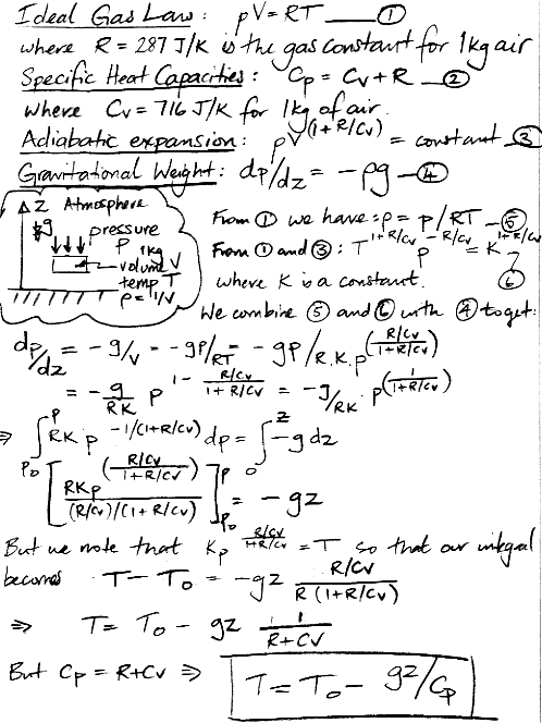
We see that the temperature of an atmosphere stirred by convection must drop linearly with altitude. Michele has proved this to us a number of times, in different ways. The differential form of the result is:

dT/dz = − g/Cp
For dry air on Earth, we have g = 10 N/kg and Cp = 1 kJ/kgK, so we expect a drop of 10 K/km. Our simulation uses cells of dry air, and it shows a drop of around 50 K from bottom to top during convection. The temperature drops to 0 K at an altitude z_T = CpT₀/g. For T₀ = 300 K we have z_T = 30 km. When the temperature drops to O K, the pressure must be zero also. With a little more pencil-work, we arrive at the following equation for pressure with altitude.

p = p₀ (1 − gz/CpT₀)^Cp/R    (for dT/dx = −g/Cp)
The pressure at the bottom of our cell array is 100 kPa, and at the top is 50 kPa, with the bottom temperature at 300 K. The height of our array is 5.4 km, giving the simulation an average temperature drop of close to 10 K/km. In Atmospheric Pressure, we considered an atmosphere at uniform temperature, and arrived at the relation:

p = p₀e^−gz/RT    (for dT/dx = 0)
The atmosphere with uniform temperature never comes to a definite end, but keeps getting thinner and thinner with altitude.


Figure: Pressure versus Altitude for Constant Temperature (dT/dz=0) and Adiabatic Convection (dT/dz=−g/Cp) with T₀ = 300 K and p₀ = 100 kPa. The mass of the atmosphere is p₀/g = 10,000 kg/m² in both cases.
When our cell array is at a uniform temperature T = 250 K, the height of the array will be 5.0 km. Warming the atmosphere to initiate convection causes the top to rise by 400 m.

The −gz/Cp slope of the temperature profile is called the dry adiabatic lapse rate. The Earth's atmosphere is not dry. As moist air expands and cools, water condenses, which releases heat. Thus the wet adiabatic lapse rate is less than the dry adiabatic lapse rate. The lapse rate in the Earth's atmosphere appears to be 6 K/km.

Convection takes place when the temperature drops linearly with altitude. In an atmosphere stirred by convection, gravitational potential and atmospheric temperature are intimately related. A change in one will be matched by an equal and opposite change in the other.

Surface Cooling, Part VI

We continue our study of Surface Cooling with the help of Circulating Cells, Version 5. We consider the transport of heat from a hot, sandy surface into the interior of a three-hundred meter cube of air. This three-hundred meter cube represents a single cell in the bottom row of our Rotating Greenhouse simulation. We refer to this cube as our super-cell. We are going to divide it into an array of sub-cells and heat the bottom row of sub-cells so as to induce convection within the super-cell.

We start by modifying our CC5 program. We set p_bottom to 100 kPa and p_top to 96.7 kPa. The total mass of our cell array is now 330 kg/m², which is the mass of our super-cell. The program will create an array of sub-cells with 30 columns and 15 rows. Each sub-cell will have mass 20 kg/m² and be 17 m high.

We set T_initial to 290 K, which is typical of a super-cell freshly-arrived at the surface our Rotating Greenhouse. We select Surface Heating, which warms the lowest sub-cells at a constant rate but allows no heat to escape from the array. According to our previous calculations, our super-cell will start to rise when it has warmed by a few degrees. Until then it will accumulate heat by convection of its own sub-cells.

When we start CC5, it calculates a value for the sub-cell impetus threshold using the procedure we describe in Impetus for Circulation. This value turns out to be 0.00003 K, a thousand times smaller than the value CC5 calculates for super-cells in our Rotating Greenhouse. As we showed in Simulation Time, each iteration of our simulation represents one second of planetary time. The heat arriving from the sun in the middle of the day can be as high as 1.4 kW/m². Let us suppose our sandy planet surface is receiving 800 W/m². The sub-cells have mass 20 kg/m² and heat capacity 1 kJ/kgK. We set Q_heating to 0.04 K so that the bottom sub-cells warm at 0.04 K/s. We set our mixing fraction to 0.10. Each time a sub-cell circulates, it will exchange one tenth of its volume with its neighbors.

We reset the sub-cell array and start running. The Figure below shows the simulation after about an hour of simulated time (four thousand iterations).



We record the average temperature of our sub-cell rows and obtain the following plots.



After half an hour, the bottom row of sub-cells has warmed by 20 K and the row above has warmed by 15 K. Meanwhile, the average temperature of all the sub-cells taken together has risen by 5 K. Once it has warmed by 5 K, the super-cell is likely to rise away from the surface, so further warming will be prevented.

The sub-cells above the surface warms by ten or twenty degrees during the day. This warming provides the impetus for the local convection we proposed in our previous post. At the end of the day, sub-cell convection stops, and super-cell convection brings cool air down from above.

And so our simulation confirms the process we described in Surface Cooling, Part III. After sunset, the air temperature in a sandy desert will cool by twenty degrees within a couple of hours. Furthermore, the temperature we experience standing on the sand at mid-day will be twenty degrees warmer than the temperature of the air three hundred meters up.

Rotating Greenhouse

The Rotating Greenhouse configuration of Circulating Cells, Version 5 simulates the cycle of day and night that results from the rotation of a Planetary Greenhouse with respect to its sun. The day_length_hr parameter gives the length of the day-night cycle in hours. In Simulation Time, we concluded that one iteration of our simulation corresponded to one second of planetary time, so one hour is 3600 iterations and one twenty-four hour day is 86400 iterations. The sun will shine upon our Rotating Greenhouse for a fraction of the day given by day_fraction. You will find both parameters in CC5's configuration array.

As in the Planetary Greenhouse, the surface is something like sand. It heats up quickly and warms the bottom cells of the atmosphere. Now that the planet is rotating, the heat from the sun increases from zero at dawn to a maximum at mid-day, and decreases to zero again at sunset. We use a sinusoidal profile for the rise in solar heating during the day. For the entire night, no heat arrives at all. In the middle of the day, heat arrives from the sun at a rate π × Q_heating. When day_fraction is one half (the days and nights are of equal length), the average rate at which the bottom cells are warmed by the sun is Q_heating. But when the day is shorter, the average warming is less than Q_heating, and when the day is longer, the average warming is greater. For now, we leave the fraction at one half.

The top cells, meanwhile, radiates heat into space just as they did for the Planetary Greenhouse. Top cells cool by Q_heating per second when they are at temperature T_balance. Their cooling rate increases as the fourth power of their temperature.

We allow the Rotating Greenhouse simulation to run. The report line gives us the time in hours instead of the iteration counter. In the top-left of the report window we see the current rate of solar heating, in units of K/hr. After many days, the cycle of day and night reaches equilibrium, and we see the following each day.



During the day, the surface cells warm as they absorb the Sun's heat. Once they warm by a few degrees, they rise, as we describe in Impetus for Circulation. The average temperature of the surface rows rises by a few degrees during the day, but not more. Our simulation does not allow surface cells to cool. And yet the average temperature of the surface row drops by a few degrees at night. When we mark a few cells near the surface, and watch them move after night falls, we see the surface cells being replaced by cooler cells from above. It is air descending from above that cools the surface row. And so our simulation confirms the mechanism for surface cooling we described in Surface Cooling, Part III.

Our simulation does not, however, show the sudden ten-degree cooling we observe standing in the desert just after the sun sets. Understanding this sudden drop was the motivation behind our Surface Cooling series of posts. Next time, we will use CC5 in its Surface Heating configuration to simulate the transport of heat within one or our large surface cells, and so obtain an estimate of how much the first twenty meters of the atmosphere will warm up during the day.

PS. You will find the array data corresponding to the start of the day with Q = 0.001 K and no cell mixing in RGH_Q001

Impetus for Circulation

Today we introduce Circulating Cells, Version 5. You can download the source code here. As usual, you will find instructions for running the program in the comments at the top. The source code is text file, so you can open it with any text editor. We have removed the Mix check box in CC5. You now turn off the cell mixing by setting the mixing fraction to zero.

Today's post is longer than usual. We present a mystery that we would like you to help us solve, but we also describe what happens to our simulation when we try to make sure that cell circulations take place quickly enough to be consistent with simulation time.

In Work by Circulation we showed that the rising cell does more work in the act of expanding than is required to compress the falling cell. This excess work will accelerate the cells so that they circulate. If the expanding cell cools by 3.032 K and the falling cell warms by only 3.000 K, the missing 0.032 K represents heat and pressure energy that has been converted into work. With heat capacity 1 kJ/kg, there will be 32 J of work available for each kilogram of gas in the rising cell. When divided between the four cells, there will be 8 J/kg. We call this the expansion work.

Convection occurs in water as well as air. Water at 20°C is 0.2% less dense than water at 4°C. A cell of water at 20°C will be buoyant within water at 4°C. We often think of water as an incompressible fluid. But it is slightly compressible. Water at 100 kPa is 0.004% less dense than water at 200 kPa. Water at 20°C rising from a depth of 10 m to the surface of a lake will do 6 mJ/kg of work by expansion. Meanwhile, water at 4°C falling from the surface to a depth 10 m will require 0.2% less work for its compression. The excess 12 μJ/kg is adequate to accelerate four equal cells to 2.5 mm/s. It is conceivable, therefore, that expansion work can power convection in water.

Nevertheless, there appears to be another source of work to power circulation. In a block of four cells, if we have a hot cell on the lower-left and a cold cell on the upper-right, the block's center of mass will descend when we rotate clockwise. The upper-left cell slides off the hot cell to rest upon the cold cell. As it slides, the top-left cell pushes the other three cells around to complete the circulation. The circulate routine of CC4 calculates how far the center of mass of a block of four cells will descend if we rotate the block by a quarter-turn. We describe this calculation in a comment here. If the block's center of mass drops by 0.8 m in gravity 10 N/kg, the weight of the block will provide 8 J/kg of work. We call this the buoyancy work.

In CC3 we rotated a block of cells only if the buoyancy work was positive. We ignored the effect of expansion work and buoyancy work upon the cells. Of the heat we put into the array at the bottom, only 85% emerged from the top by radiation. In CC4 we calculated the expansion work and divided it up between the four cells to represent viscous heating. At equilibrium, 100% of the heat we put in emerged from the top. Our simulation conserved heat, but it ignored buoyancy work. How can that be?

Furthermore, how large is the buoyancy work compared to the expansion work? If one is positive, is the other always positive? The circulate routine of CC5 includes code that calculates both the buoyancy work and expansion work, and reports them both. We ran our simulation with this code activated. In a wide variety of conditions, both evolving and convergent, the buoyancy work was always between 95.7% and 97.6% of the expansion work. To within the margin of error introduced by our simulation, buoyancy and expansion work are equal.

Why are they equal? Michele has proved to me several times that for adiabatic circulation, temperature will drop linearly with altitude. Could it be that this linear relationship causes buoyancy and expansion work to be equal? Or are buoyancy work and expansion work just two faces of the same process, so that we can count one or the other, but not both? If they are one and the same, then buoyancy work cannot exist without expansion work, which implies that convection would not occur in a perfect, incompressible fluid. But surely convection can occur in a perfect, incompressible fluid?

We would like to provide you with answers to these questions, but we don't have them yet. Perhaps, after a few more debates with Michele and anyone else who wants to take part, we will have answers. For now, however, we are going to assume that we cannot add buoyancy and expansion work together to obtain the total work available to accelerate our cells. We have a simulation that conserves heat at equilibrium, and we want to keep it that way. We will calculate and use the expansion work only, and add it back to the cells as viscous friction.

In the circulate routine of CC5, we calculate the drop in the combined temperature of the four cells in a block. We call this net loss our impetus for circulation. If the impetus is 0.032 K, our expansion work will be 8 J/kg when spread among the four cells. The cells could, in theory, reach a speed of 4.0 m/s. The cells in our atmospheric array are roughly 400 m high, so a circulation at 4 m/s will take place in 100 s. There are 450 cells in our 15×30 array, and our simulation picks a new block on every iteration. We expect one of the four cells in our block to be picked again within a hundred iterations. But one hundred iterations corresponds to 100 s, so we see 0.032 K is the minimum impetus required to make sure that our rotation takes place before we expect one of its cells to take part in another rotation.

Our CC5 program rotates a block of four cells only if its impetus for circulation is greater than an impetus threshold. With the impetus threshold set to 0.032 K, we ran CC5 to produce new versions of the graphs we presented in Simulation Time.



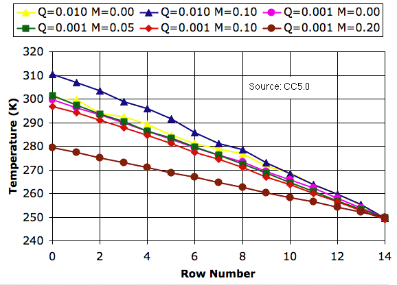
The impetus threshold has no effect upon the profiles we obtain with no mixing (M = 0.0). Nor do we see any effect with heavy mixing (M = 0.20). We do, however, see a slight change in the presence of mild mixing (M = 0.05). Mild mixing now raises the surface temperature by a few degrees.

The impetus threshold makes sure that rising cells are significantly warmer than falling cells. When a cell rises from row 7 to row 8, its temperature drops by a factor of 0.9879 (see here). If our impetus threshold is 0.03 K, warm cells about to rise from row 7 must be 0.03 K ÷ (1-0.9879) = 2.5 K warmer than cool cells about to arrive in the same row. Between the bottom rows, the required difference is 3.0 K, and between the top rows it is 1.7 K. With Q = 0.001 K, a cell freshly-arrived in the bottom row will warm by 3.0 K in three thousand iterations, which is almost an hour. Soon after, it will start to rise.

In our next post, we will see how well our program performs when we simulate night and day using CC5's new Rotating Greenhouse configuration.

PS. You will find the equilibrium array for Q = 0.001 K and M = 0.00 in PGH_Q001_M00. The array for Q = 0.001 K and M = 0.20 is PGH_Q001_M02. Saved arrays now have comments in them that tell us the conditions under which they were obtained.

Summary to Date

On the side-bar, you will see a new link, Summary to Date. The new page gives a history of the posts on this site. It attempts to explain what we have achieved so far, what we are working on now, and what we hope to achieve in the future. I'll maintain the page, adding paragraphs every few months. With any luck, the page will allow newcomers to make sense of what's going on.