Water Vapor Continuum

It may be that we can determine the absorption length of long-wave radiation in dry air with 330 ppm CO2 simply by dividing the absorption length pure CO2 by 0.00033. The absorption length of 15-μm radiation in pure CO2 is 10 mm (see CO2 Spectrum), so its absorption length in 330 ppm by volume CO2 would, according to this calculation, be 30 m.

The absorption spectrum of water vapor is not so simple. We have already presented our readers with the absorption spectrum of liquid water. But we cannot simply divide this spectrum by the fraction of water present in air and so obtain the spectrum for water vapor. Water vapor is water dissolved in air. The spectrum of liquid water applies to the Earth's oceans, and to the tiny droplets of water in clouds, but it does not apply to water vapor, as we saw in Vapor Versus Liquid. Water vapor absorbs several orders of magnitude less long-wave radiation than we would expect from dividing the liquid water spectrum by the water vapor concentration.

In liquid water, there are hydrogen bonds between each water molecule and its neighbors. These bonds absorb long-wave radiation. Hydrogen bonds are far less common in water vapor because the molecules are separated. Hydrogen bonds occur in water vapor when pairs of molecules join together to form dimers. The hydrogen bonds in these dimers absorb long-wave radiation. The chance of a water molecule finding a partner to form a dimer increases with concentration. At the same time, the number of water molecules per unit volume increases with concentration. The result is that the absorbing power of water vapor increases as the square of the concentration. Absorption by water vapor is also temperature-dependent because dimers are broken apart by kinetic energy, so colder dimers live longer and have more opportunity to absorb long-wave radiation.

There are also weak long-wave absorbing bonds between water and nitrogen, and water and oxygen. The absorption of long-wave radiation by water vapor is an on-going subject of research at many institutes. The relationship between molecules in water vapor is called the water vapor continuum. In Water vapor absorption coefficients in the 8−13-μm spectral region: a critical review (1990), Grant et al review existing measurements of the water vapor continuum spectrum. In Recent Developments in the Water Vapor Continuum (1999), Mlawer et al review existing calculations of the spectrum. The following graph of water vapor continuum absorption agrees well with measurements such as these.



Instead of plotting the spectrum versus wavelength, this graph plots the spectrum versus the inverse of the wavelength, in units of cm⁻¹. The spectrum itself takes the form of a quantity in units of cm² molecule⁻¹ atm⁻¹, plotted for various temperatures between 220 K and 330 K. In our next post, we will convert this graph into one of absorption length versus wavelength, and show how we can calculate the absorption of long-wave radiation by water vapor in the atmosphere.

PS. Thanks to Peter Newnam for his help researching this post.

UPDATE: See CO2 Continuum for the spectrum of diluted CO2.

CO2 Doubling Temperature

One claim made by climatologists is that each doubling in the concentration of CO2 will cause the same increase in the Earth's surface temperature. So far as we can tell, the basis for this claim is that the absorption of radiation by greenhouse gases is "logarithmic". See Nelson, Earthguide and Wikipedia for examples. We never understood this "logarithmic" argument. We have never seen any calculations to back it up.

The greenhouse effect in our Planetary Greenhouse example is the result of logarithmic absorption by a greenhouse gas. The atmosphere contains a hypothetical gas that is opaque to some, but not all, long-wave radiation. As we showed in our previous post, successive doublings in the concentration of this gas do not cause the same increase in surface temperature. Indeed, the graph produced by our computer program shows that each successive doubling causes half as much warming as the previous doubling.

Thus logarithmic absorption alone is not sufficient justification for the existence of a "CO2 Doubling Temperature".

Planetary Greenhouse, Part Two

We continue our Planetary Greenhouse discussion. The atmosphere around our imaginary planet contains nitrogen and oxygen, which we choose because these diatomic gases are transparent to both short-wave and long-wave radiation. But the atmosphere also contains an imaginary greenhouse gas that is transparent to wavelengths shorter than λ_T, but absorbs longer wavelengths with constant absorption length, L_T.

We wrote a computer program to determine the total heat radiated per square meter by the planet and its atmosphere. Before we can run the program, we must choose λ_T and L_T.

Consider the absorption spectrum of pure CO2 at roughly 300 K and 100 kPa, which we present here. Between 8 μm and 11 μm the gas is transparent. The graph of radiated power versus wavelength for a black body at 300 K, which we present here, shows a peak at around 10 μm, right in the middle of CO2's transparent band. Meanwhile, the gas is at its most opaque for wavelengths greater than 13 μm. The absorption length drops to as little as 1 cm between 13μm and 17 μm, but is close to 1 m for 17 μm and higher. Let us choose λ_T = 13 μm and L_T = 1 m.

Suppose our greenhouse gas makes up 330 ppm by volume of the atmosphere around our imaginary planet. Suppose the pressure at the planet surface is 100 kPa and the temperature is in the neighborhood of 300 K. The absorption length of the atmosphere at at the surface will be 1 m / 330 ppm = 3 km for wavelengths greater than λ_T. In The Upper Gas we showed how the absorption length at the surface is related to the pressure in the tropopause. With absorption length 3 km at the surface, the tropopause pressure will be 30% of the pressure at the surface, or 30 kPa. If we double the concentration of the greenhouse gas from 330 ppm to 660 ppm, the absorption length at the surface decreases to 1.5 km, and our tropopause must rise to an altitude where the pressure is only 15 kPa.

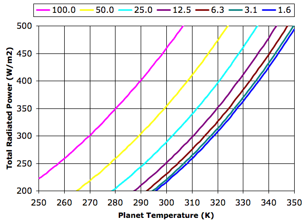
Now we can run our program, and we do so. We calculate the sum of the power radiated directly into space by the planet surface and by the troposphere. We plot this total radiated power versus the temperature of the planet surface, and we do so for a range of tropopause pressures.



The graph legend gives tropopause pressure in kPa. Each halving of pressure corresponds to a doubling in greenhouse gas concentration. The 100 kPa graph represents the case where the concentration is so low that the troposphere is at the planet surface. The planet radiates like a black body directly into space. The 1.6 kPa graph represents a concentration so high that the the troposphere radiates hardly any heat into space. The atmosphere acts to block all radiation at wavelengths greater than λ_T.

For thermal equilibrium in our Planetary Greenhouse, the total power radiated into space, E_P + E_T, must be equal to the total power received from the sun, E_S. In Solar Heat we showed how the average power reaching the Earth from the Sun was 350 W/m², and we calculated that the surface of a black planet with no atmosphere would be 280 K. In the 100 kPa graph above, we see that the surface temperature, T_P, crosses 280 K when the total radiated power is 350 W/m².

Let us suppose that the total radiated power in our Planetary Greenhouse must be 350 W/m². With a tropopause pressure of 50 kPa, the planet surface must be at 299 K. If we double the concentration of our greenhouse gas, the planet warms by 13 K. Subsequent doublings in concentration raise the temperature by an additional 7 K, 5 K, 3K, and 1 K.

Planetary Greenhouse

We now enhance our Extreme Greenhouse to produce a more interesting model. We incorporate the decrease in atmospheric pressure with altitude. We use our understanding of atmospheric convection to determine how atmospheric temperature changes with pressure. We enhance the properties of our greenhouse gas by making it transparent to some long-wave radiation. The result is a simple model of a Planetary Greenhouse, as shown below.



In our new model, the atmosphere continues to infinite altitude, getting thinner and thinner as we go. The lowest layer of the atmosphere is the troposphere. Above the troposphere is the tropopause. The tropopause is the layer that radiates heat into space. Above the tropopause, the atmosphere is so thin that it is transparent.

For now, we ignore day and night, and we ignore clouds. We ignore heat flowing through the solid mass of the planet. Short-wave radiation arriving from the sun passes straight through the atmosphere and is of uniform and constant power E_S. The temperature and pressure at the planet surface are T_p and P_p respectively. A near-adiabatic convection cycle carries heat up through the troposphere to the tropopause, where it is radiated into space. The temperature and pressure of the tropopause are T_T and P_T respectively.

In our Extreme Greenhouse, the atmosphere was entirely opaque to all long-wave radiation. In our new Planetary Greenhouse, the atmosphere is transparent to all radiation with wavelength less than some threshold, λ_T. At greater wavelengths, a trace greenhouse gas in the atmosphere absorbs radiation. The greater the concentration of this greenhouse gas, the shorter the absorption length of the atmosphere for wavelengths greater than λ_T. As we saw in The Upper Gas, the shorter the absorption length, the lower the tropopause pressure. As we saw in Atmospheric Convection, the lower the tropopause pressure, the lower its temperature.

As in our Extreme Greenhouse, we assume that the planet radiates like a black body. The radiation it emits below λ_T passes out into space. This radiated power is E_P. As we described in Black Bodies, we can use Plank's Law to determine the power radiated at all wavelengths, so we can calculate the power radiated below λ_T as a function of T_P.

The atmospheric convection cycle allows us to calculate the temperature of the tropopause given only T_P and the ratio P_T/P_P. The tropopause radiates power E_T into space. Using Plank's Law and radiative symmetry, we can calculate the power radiated by the tropopause as a function of T_T. The atmosphere emits radiation only at wavelengths greater than λ_T.

For thermal equilibrium, we must have the total power radiated outward by the body and the tropopause equal to the total power arriving from the sun. Thus we must have E_S = E_P + E_T. And so we arrive at a robust model of the planetary greenhouse effect when the greenhouse gas has a step-like absorption spectrum. Given only λ_T and P_P, we can plot a graph of E_P + E_T versus temperature. This graph crosses E_S at the equilibrium value of T_P. We wrote a computer program to calculate E_P + E_T versus T_P for a range of tropopause pressures. You will find the program here.

In our next post, we will choose useful values for λ_T and E_S, and we will see how doubling the concentration of our greenhouse gas affects the temperature of the planet.

Dissipation by Convection

Now we return to our Extreme Greenhouse thought experiment. In our previous post on the subject, Work by Convection, we showed that atmospheric convection does work. We wondered where the energy for that work comes from, and where it goes to.

In our Atmospheric Convection post, the air taking part in our convection cycle warmed by 15 K while in contact with the warm surface of the Body, and cooled by 10 K while in the tropopause radiating its heat into space. The warming and cooling took place at constant pressure. The amount of heat required to warm 1 kg of a gas by 1 K at constant pressure is the heat capacity at constant pressure of the gas. Air is a close to an ideal gas. Its heat capacity at constant pressure is close to 1 kJ/kg/K at all the temperatures and pressures we are likely to encounter in the atmosphere of our Extreme Greenhouse. Each 1 kg of air absorbs 15 kJ of heat from the Body and radiates 10 kJ of heat into space. There are 5 kJ unaccounted for. These 5 kJ are converted into work.

Each kilogram of air taking part in the cycle rushes upwards with such force that it will do 5 kJ of work for us and still reach the tropopause. As it rushes upwards, it mixes with other air. Its momentum is diverted into whirlwinds. The viscosity of air is low, but it is not zero. The air moves upwards and sideways and in circles, rubbing against itself until the viscous friction it encounters consumes all the work available from convection. Viscosity turns the 5 kJ into heat.

As a result, the air in the tropopause will be warmer by 5 K than we expected with perfect, adiabatic expansion. Given that the air in the tropopause is over 100 K cooler than the air at the surface of the Body, this 5 K makes little difference to the size of our greenhouse effect. But it does mean that the air must cool in the tropopause by 15 K instead of 10 K, or else our convection cycle will not be closed. All 15 kJ of heat absorbed by the air from the Body will be radiated into space at the tropopause.

We know from our previous calculations that the atmosphere of our Extreme Greenhouse must transport 350 W/m² from the Body surface to the tropopause (the boundary between the Filter Gas and the Upper Gas). Of these 350 W/m², roughly 230 W/m² will be carried directly by the heat capacity of the atmosphere, but the remaining 120 W/m² will first be turned into work, later converted into heat by viscous action, and finally radiated into space.

The atmosphere of our Extreme Greenhouse has 120 W/m² available to cause weather. This work is available only because the upper atmosphere is radiating heat into space. If there were no greenhouse gases in our Extreme Greenhouse, there would be no heat flow to the upper atmosphere, and no convection cycle to generate weather.

CO2 Sequestration

Peter Newnam points us to an article in The Guardian discussing the implications of a recent paper, Sequestering Carbon Dioxide in a Closed Underground Volume by Economides et al. We do our best to present the content of the paper in the following paragraphs, because we cannot see the content explained anywhere else. For consistency with our other posts, we will convert the paper's imperial units to metric units.

One way to get rid of CO2 is to pump it into the ground and leave it there. Storing CO2 under the ground is called carbon dioxide sequestration. If we pump CO2 into the ground just any old place, it will leak out again. We must find a suitable geological formation that will hold and keep the CO2 indefinitely. An aquifer is an example of such a formation: a layer of permeable rock, perhaps a hundred meters thick, surrounded on all sides with impermeable rock. Aquifers are usually filled with water, oil, or natural gas.

Exhausted oil reservoirs are ideal aquifers in which to store CO2 because they have been depleted of their fluid content. Oil companies even go so far as to buy CO2 and pump it down into oil reservoirs to push the oil out. But exhausted oil reserves are already being used to store natural gas. They are not available for sequestration. Most CO2 sequestration schemes use an aquifer that is saturated with water or brine. We pump the CO2 into the aquifer at sufficient pressure to compress the water and the rock. The rock and water get smaller to make space for the CO2.

The initial pressure of almost all aquifers, before we start pumping in CO2, will be close to Hρg, where H is the aquifer depth, ρ is the density of water, and g is gravity. An aquifer 2 km down will have formation pressure close to 20 MPa = 200 Bar. Aquifers fracture if the pressure gradient from the surface to the aquifer exceeds 20 kPa/m. An aquifer at 2000 m cannot be pressurized to more than 40 MPa = 400 Bar without fracturing. When an aquifer fractures, its contents leak out.

Suppose the aquifer is initially 20% water and 80% rock. The bulk modulus of rock is roughly 70 GPa and of water is roughly 2 GPa. If we raise the pressure in the aquifer from 20 MPa to 40 MPa, the volume of the pre-existing rock and water shrinks by 0.36%. The Prudhoe Bay reservoir is the largest oil field in the United States. It is 1000 km² in area and up to 100 m thick. Suppose our sequestration reservoir is of the same size. When we pressurize it to 40 MPa, the 10¹¹ m³ volume of the aquifer's rock and water contracts by 360×10⁶ m³. Meanwhile, CO2 at this pressure has density 650 kg/m³, so the maximum mass of CO2 we can store in our aquifer without fracturing its impermeable rock walls is 240×10⁹ kg. A 500-MW coal-burning power plant produces 3×10⁹ kg/yr. There are roughly one thousand such coal-burning plants in the US alone. One thousand reservoirs the size of Prudhoe Bay would be required to store the CO2 generated by these one thousand plants over the course of eighty years.

But the paper shows that the capacity of an aquifer is further limited by the rate at which we can inject CO2 into the aquifer. In order to force CO2 through the the porous rock, we must apply a pressure greater than the reservoir pressure, and even with 10 MPa of excess pressure, the CO2 does not rush into the aquifer. It seeps in. An aquifer five times the size of Prudhoe Bay, along with four separate injecting wells, would be required to sequester the CO2 produced by a single 500-MW coal-burning power plant.

Previous work on the subject suggested that we could push CO2 into an aquifer ten to a hundred times faster. Economidese et al. mention two problems with previous work. One problem is that previous work confused the volume of the pores in the aquifer with the volume of the aquifer. The volume of the pores is only 20% of the volume of the aquifer. This confusion led to an over-estimation of the sequestration rate by a factor of five. The other problem is that previous calculations assumed that the pressure at the boundaries of the aquifer was constant. If the pressure at the boundaries is constant, we certainly can push CO2 in faster, perhaps ten times faster. But such an assumption implies that water, and ultimately CO2, will escape the aquifer at the boundaries. In other words: you can fit a lot more CO2 into an aquifer if you allow it to leak out at the edges, but that rather defeats the purpose of sequestration.

In short: the paper concludes that carbon sequestration is impractical. The state of Rhode Island would require an aquifer as large as itself just to sequester 20% of the CO2 generated by its own electricity consumption.

UPDATE: My father is a retired chemical engineer. He was a pioneer in liquified natural gas. He designed the large LNG tank outside Boston, where I live. He also studied CO2 sequestration twenty-five years ago. He read Economides et al. and "did not think much of it". He says there are better places to put CO2 than the aquifers discussed in the paper.

Committees and Law Suits

Michael Mann, of Mann-Made Warming, has hired a law firm. His law firm wrote to Minnesotans for Global Warming (MGW), the makers of the Hide the Decline music video. This video uses a photograph of Dr. Mann's face. The letter from the lawyers demands that MGW stop using Dr. Mann's likeness, saying the "video clearly defames Professor Mann by leaving viewers with the incorrect impression that he falsified data to generate desired results". Youtube has removed all copies of the video, as well as a new version that does not use Dr. Mann's face. But No Cap and Trade is still hosting the original video, which I linked to earlier in this paragraph.

If Dr. Mann goes to court with MGW, his lawyers will argue that he did not fabricate measurements or data. But the defense will be able to address the definition of "data" and "measurement", and so shine light upon the idea of "value-added data" and "multi-proxy statistics". Dr. Mann combined measurements in a way that created a hockey-stick graph regardless of the input data, and even goes so far as to invert measurements that decline, so they rise instead, and contribute to the hockey-stick shape. Dr. Mann presented his Hockey Stick Graph as if it were a measurement. Either he knew full well that he was falsifying this measurement, or he became confused and did not understand his own mistake. Subsequent inquiries prompted by the work of Mr. McIntyre gave Dr. Mann ample opportunity to see his error and withdraw his graph. But Dr. Mann still insists that his graph is a useful measurement of global temperature changes over the past thousand years.

A law suit bestows the power of subpoena. Dr. Mann could be interrogated in court or during depositions. He would have to answer questions about his work. He would not be able to dismiss the inverted-measurement accusation as "bizarre" and say nothing more about it. So I hope the case goes to court. I would donate to the MGW legal fund.

Here's another law suit. Climate modeler Andrew Weaver asked Canada's National Post to "retract a number of recent articles that attributed to me statements I never made, accused me of things I never did, and attacked me for views I never held." Perhaps Mr. Weaver is referring to articles like this, in which he comes across as a conspiracy theorist. The National Post refused to retract their statements, so Mr. Weaver is suing them for "grossly irresponsible falsehoods" and for insults posted in the on-line comments.

Mr. Weaver's case looks like it will degenerate into an argument about what he said in interviews, not an argument about the science. So I'm not as enthusiastic about his law suit. I hope the paper did not misrepresent him. I image being misrepresented must be frustrating.

A second inquiry into Climategate has produced its conclusion. This inquiry was headed by Lord Oxburgh and was instigated by the University of East Anglia, home of the Climatic Research Unit (CRU) and epicenter of the entire affair. The inquiry concluded that the scientists involved did nothing wrong. This conclusion has been greeted with enthusiasm by most climatologists, such as those providing content at Realclimate, but there are some climatologists who are not satisfied by either the Oxburgh Report or the Parliamentary Report. Vocal among the critics of these reports is Judith Curry. She notes, and we agree with her, that neither report addresses any of the main issues raised by critics of climate science, such as those listed in by Mr. McIntyre in his submission to the Parliamentary Committee. But the two inquiries were supposed to identify any "wrong-doing" on the part of CRU scientists. I'm not sure what "wrong-doing" is.

The point of Climategate is that climatologists don't obey the same rules as the rest of us in other fields of science. We don't substitute instrument data for proxy data and then plot the result as if it were all proxy data (Gavin Schmidt). If I were to hide a trend using a trick, I would deserve to be fired from my position. It's not up to committees to condemn climatologists. It's up to us scientists in other fields to distance ourselves from their work so that their field can no longer lay claim to the authority that has been earned by properly-conducted science over the past three centuries.

These law suits hold more promise than the committees. In the law suits, the definition of scientific conduct would be addressed, and judges are good at understanding the logic of definitions. Let's not forget the great work done by Judge John E. Jones on the subject of intelligent design. He judged that the definition of "science" was that it addressed natural phenomena only, so any theory, such as intelligent design, which mentioned the existence of a super-natural being, was by definition non-scientific, regardless of its truth or falsehood. We need a judge like him in the Dr. Mann vs. MGW case.