Tuesday, February 22, 2011

Circulation and Mixing, Part II

The blue plot in the graph below shows the temperature of a single cell performing a complete circulation within our Planetary Greenhouse simulation. The cell exchanges no heat with its neighbors. We have mixing fraction zero, Q_heating at 0.01 K, and T_balance at 250 K. The cell warms up in the bottom row (the Sun heats the surface) and cools down in the top row (the tropopause radiates into space).


In any given row of the atmosphere, the cell is 20 K warmer on the way up than on the way down. Even though a rising cell may pass by a falling cell, they exchange no heat. The convection is adiabatic. The average temperature of the bottom row is roughly 50 K warmer than the average temperature of the top row.

Now suppose we allow the passing cells to exchange heat. The warm, rising cells cool down because they mix with the cool, falling cells. In order to reach the top, a cell will have to start off hotter than it would without mixing. Cells rise part-way, mix with their neighbors, fall, and mix with their neighbors again. The pink plot shows the variation in temperature, with mixing fraction 0.4, as a cell rises and falls during a hundred thousand iterations of the simulation. The average temperature of the bottom row is roughly 70 K warmer than the top row.

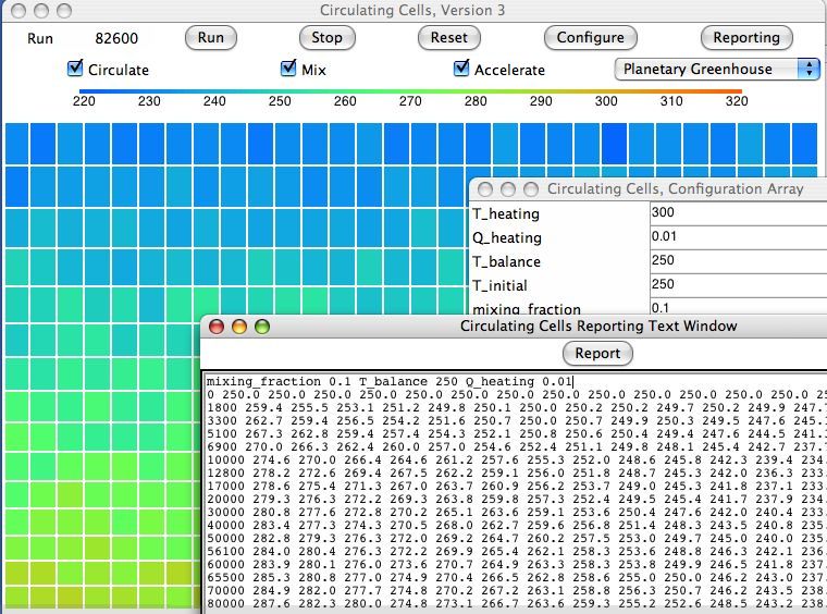
The following plot shows how bottom-row temperature varies with mixing fraction for Q_heating at 0.01 K. (Thanks to Peter Newnam for the data.) As we increase the mixing, circulation is further impeded, but but the mixing itself begins to transport sufficient heat to bring down the surface temperature.


Circulation alone is an efficient transporter of heat. The following plot shows that we see little change in the atmospheric temperature profile as we increase Q_heating by a factor of ten from 0.01 K to 0.1 K. The profile for 0.1 K is erratic, but on average is almost the same as that for 0.01 K.


When we allow mixing, we break up the continuous circulation that would otherwise transport heat from the surface to the tropopause. Instead of one continuous circulation we have a series of circulations carrying heat up in stages. Heat transport between stages takes place by mixing. The average temperature of the surface must increase because heat exchange by mixing requires an additional temperature drop over and above the adiabatic temperature drop produced by circulation.

To round off our explanation of the effect of mixing, imagine a continuous circulation from bottom to top consisting of two parallel columns of cells. One column is rising as the other falls. Now we suppose that each rising cell must be 10 K warmer than its side-by-side neighbor in the falling column, or else circulation will stop. Furthermore, we suppose that each time the circuit rotates by one cell, we allow some mixing between the side-by-side neighbors. The rising cell cools by 1 K and the falling cell warms by 1 K. Because of this mixing, a cell that has just descended will be 1 K warmer than without mixing. If it is to be 10 K cooler than its new side-by-side neighbor, this neighbor must be 1 K warmer than in circulation without mixing. The 10-K difference between the side-by-side neighbors in the column will be sustained only if the total temperature drop from bottom to top increases by 1 K multiplied by the number of cells from bottom to top. In our case, that would be 15 K.

Mixing raises the temperature difference necessary to transport heat through the atmosphere. The temperature difference is therefore greater than that dictated by adiabatic convection alone. In future posts we will enhance our simulation to allow cells within the array to radiate heat directly into space. This radiation, taking place before the cells reach the tropopause, will decrease the temperature drop between the bottom and the top. For now, however, we are satisfied that our program is effective in its simulation of mixing and circulation.

Monday, February 14, 2011

Circulation and Mixing, Part I

We run CC3 program in Planetary Greenhouse mode with mixing_fraction = 0.1, Q_heating = 0.01 K, and T_balance = 250 K. The following graph shows the average temperature of the top and bottom rows versus iteration, which is the simulation's version of time. The entire array starts off at 250 K.


The top row represents our simulated planet's tropopause. We see the top row cooling during the first ten thousand iterations as it radiates its heat into space. At the same time, the bottom row warms up as it absorbs heat from the Sun. After the first ten thousand iterations, convection starts to transport this heat away from the bottom row and deliver heat to the top row. The pace of warming and cooling slows down. After a few hundred thousand iterations, the top row settles at 239 K while the bottom row settles at 297 K. When we watch the simulation, we see cells rising to the top, cooling, and sinking to the bottom in convection cycles. Now that thermal equilibrium has been reached, we know that the top row must be losing heat at the same rate that heat enters the bottom row.

Because we set T_balance to 250 K, we know the top row in our simulation will radiate as much heat as is arriving from the sun when its cells are all at 250 K. But the top cells radiate heat in proportion to the fourth power of their temperature. Furthermore, the temperature of the upper cells is not uniform. Cells arriving from below are warmer. Those that are warmer will radiate disproportionately more than those that are cooler. As a result, the average temperature of the top row can be less than 250 K. We will consider this effect in more detail later. Today we want to present the effect of mixing upon circulation. (UPDATE: The convergence to 240 K turns out to be due to our ignoring work produced by circulation, but this omission has little affect upon the magnitude of warming caused by mixing.)

We run our simulation three times, each with a different value of mixing fraction. After a million iterations, we plot the average row temperature versus the row number, which we call the temperature profile. In the legend, Q is Q_heating and M is mixing_fraction.


With no mixing, once a cell warms up in the bottom row, no heat passes in or out until it reaches the top. In the top row, it radiates its heat into space and cools down. Without mixing, the bottom row is 49 K warmer than the top. When we allow the cells to mix with their neighbors, each cell loses heat to its cooler neighbors and gains heat from its warmer neighbors. We see that when mixing_fraction is 0.1, the bottom row warms up until it is 58 K warmer than the top row. When mixing_fraction is 0.2, it is 62 K warmer.

We might think that the exchange of heat between atmospheric cells would encourage the overall transport of heat through the atmosphere, and so decrease the temperature difference between the bottom and the top. But quite the opposite is the case. In our next post, we will endeavor to explain why. At the moment, we don't have a compelling answer. Indeed, it may be that the warming caused by mixing is nothing more than a flaw in our simulation. Your thoughts on the subject will be most welcome.

Thursday, February 10, 2011

Planetary Greenhouse Simulation

Suppose we have a planet whose atmosphere is perfectly transparent to short-wave radiation from the Sun. The surface of the planet is made of sand, which warms up quickly. It warms until it loses heat by radiation and convection as fast as it receives heat from the Sun. Meanwhile, we suppose that the lower atmosphere is opaque to long-wave radiation so all the heat from the Sun ends up in the lower atmosphere. The lower atmosphere gets hot. It rises. Like all atmospheres, this one gets thinner as we ascend. Eventually it is so thin that it becomes transparent to long-wave radiation. This layer of the atmosphere is the tropopause. The tropopause radiates heat into space according to Stefan's Law. Air in the tropopause cools until it becomes so dense that it sinks towards the surface. And so atmospheric convection begins. The heat arriving from the Sun passes into the lower atmosphere, is carried up to the tropopause by convection, and is radiated into space.

We have described such a planet and atmosphere before, in Planetary Greenhouse. Today's CC3 program simulates the transportation of heat through such an atmosphere. You can download the program here. Running in its Planetary Greenhouse configuration, CC3 supplies heat to cells in the bottom row at a constant rate. Each bottom cell heats up by Q_heating K per iteration, regardless of its temperature. Meanwhile, a cell in the top row at temperature T_balance cools by Q_heating K per iteration. At other temperatures, the cooling rate of the upper cells increases as the fourth power of the cell temperature.


In the simulation, Q_heating represents the heat arriving from the Sun. The top cells represent the tropopause, and the heat they lose is the heat radiated by the tropopause into space. The heat radiated into space by the top cells will be equal to the heat arriving from the Sun when the temperature of all the top cells is T_balance. We start the simulation with all cells at 250 K, Q_heating = 0.01 K, and T_balance = 250 K. The top cells start to cool immediately. The lower cells start to heat up.

In CC3, we corrected our implementation of heat mixing in accordance with the suggestions made by Michele. You will find our new implementation in the heat routine. We added a reporting text window, as you can see in the screen shot above. You open the window with the Reporting button. The program calls report every reporting_interval iterations, or whenever you press the Report button. We instructed report to print the average temperature of the cell rows. We added a check procedure that checks for convergence of the simulation, as requested by Peter. In the comments below I'll provide some convergence code that you can paste into the check routine. In order to accommodate the planetary greenhouse temperature variations, we doubled the breadth of the color-coded temperature range. Red is now 320 K and blue is 220 K. The Configure button allows you to change the simulation parameters while the simulation is running. Be careful not to enter invalid numbers or else the program will abort with an error.

We're running the program now. It takes several hundred thousand iterations to reach equilibrium. In our next post, will present the vertical temperature profile under various conditions. We are curious to see how the temperature of the surface is affected by the amount of heat the atmosphere must transport, and by the amount of mixing we allow between cells.

Tuesday, February 1, 2011

Mixing Cells

Our CC1 simulation allows cells to do work on one another so as to circulate by convection, but it does not allow them to pass heat to one another. The only place that heat could enter a cell was in one point along the bottom row. Today we present CC2, which allows heat to pass between cells so as to simulate mixing and conduction during atmospheric circulation. You can download the new program here.

As before, our simulation proceeds by selecting blocks of four cells at random. The simulation tests these block to see if buoyancy will cause them to rotate. In CC2, we allow heat to be exchanged between the cells of each block. We do this whether or not the cells rotate. The fraction of heat we allow to pass from each cell to each of its two neighbors is the mixing fraction. You can use CC2's new Configure button to set the mixing fraction for yourself. By default, we use 10%.

The new program provides an iteration counter, where the treatment of a block of four cells is one iteration. The display has several new buttons, as you can see below. The program starts running when you press Run. With accelerate checked, the program will update its display infrequently, so as to speed up the simulation. With the circulate and mix boxes checked, the simulation both circulates and mixes the cells. We have improved the marking of cells in this version. The marked cells have a black outline so you can see their temperature. We also increased the size of the display. Click on the following image to see the new size.


With "Point Temperature" we heat a single cell at the bottom. With "Surface Temperature" we heat all the cells along the bottom. You can set this temperature to which we heat them with the help of the Configure button.

Today we want to see how mixing affects the distribution of heat in the array with the same single-cell heating we used in our previous post. Without mixing, the cells settle down after half a million iterations to an adiabatic temperature profile, like this. With mixing the array looks pretty much the same after half a million iterations. The mixing has little effect upon the distribution of heat in the early stages of the simulation. But after 1.5 million iterations, we obtain the following array. The temperature at the top has risen from 250 K to 280 K. After two million iterations, the top of the array is at 290 K. After five million, it's above 295 K.


Half a million iterations is enough to establish an adiabatic temperature profile by convection. Five million iterations is enough to establish a uniform temperature by mixing.

We invite you to download CC2 and experiment with it yourself. For example, select surface heating to see what happens if you heat the entire bottom row of the array. Or try setting the heating temperature to 1000 K and turning off the circulation. You will see the mixing spreading heat through the array. Or run with the circulation turned on and the high heating temperature. You will see a plume of heat rising through the array.

The simulation appears to give reasonable results so far. We expected to arrive at a uniform temperature when we introduced mixing. Next time we will see what happens if we start to remove heat from the top of the array while we are inserting heat at the bottom. We wonder what type of temperature profile will evolve as heat flows up through the array.